
The problem: scaling epidemiological analysis
Epidemiologists naturally think about surveillance problems in terms of specific scenarios: “How do I detect influenza outbreaks among elderly patients in Oslo?” They develop understanding through particular cases before generalizing.
But comprehensive surveillance requires scaling these analyses across hundreds of diseases, locations, and demographic groups. Traditional programming forces epidemiologists to manage this complexity explicitly, burying analytical logic within nested loop structures:
# Traditional approach: epidemiological logic buried in scaling code
for (location in all_locations) {
  for (week in all_weeks) {
    for (age_group in all_age_groups) {
      data <- get_data(location, week, age_group)
      results <- analyze_disease_trends(data)
      save_results(results, location, week, age_group)
    }
  }
}
CS9 resolves this by separating analytical logic from scaling. Epidemiologists write code for a single instance — one disease, one location, one age group — while the framework handles expansion across all combinations automatically:
# CS9 approach: write analysis for one instance, framework scales it
short_term_trends_action <- function(data, argset, tables) {
  x <- csalert::short_term_trend(data$data, ...)
  tables$output$insert_data(x)
}
This code operates identically whether run interactively for one location or scaled by CS9 across 106 diseases, 378 locations, and multiple demographic groups. When a specific analysis fails, the epidemiologist loads that exact combination interactively and steps through the code. This is the single-instance design principle — CS9’s core innovation.
NorSySS: a decade of operation
The Norwegian Syndromic Surveillance System (NorSySS) provides evidence that this approach works in practice. Operating continuously since 2014, NorSySS has:
- Processed approximately 18 million healthcare consultations annually
- Monitored 106 diseases across 378 geographic locations (municipal to national)
- Maintained 99.5% system availability over ten years
- Supported 9 age groups and 3 sex categories for demographic stratification
During the COVID-19 pandemic (March 2020), the NorSySS team added new diagnostic codes. Within weeks the team also started to produce daily municipal-level outputs. Surveillance of the existing 106 monitored conditions continued without interruption. CS9’s single-instance design was central to this. The team developed and tested new COVID-19 analyses interactively for a single municipality. The team then deployed those analyses across all locations immediately, without additional scaling effort.
Reference: White RA, Valcarcel Salamanca B. “CS9: An analysis framework for real-time disease surveillance.” Norwegian Institute of Public Health.
CS9 vs alternatives
| Aspect | CS9 | plnr | Commercial Platforms | R Frameworks | Custom Scripts |
|---|---|---|---|---|---|
| Customization | High — domain abstractions | High — domain abstractions | Low — vendor-limited | Medium — computational flexibility | High — unlimited freedom |
| Maintenance | Low — systematic abstractions | Low — systematic abstractions | Medium — vendor dependencies | Medium — framework constraints | High — technical debt |
| User model | Epidemiological concepts | Epidemiological concepts | Standardized interfaces | Computational tasks | Complete freedom |
| Implementation speed | Medium — initial setup, then rapid | High | High — immediate capability | Medium — learning curve | Variable |
| Long-term sustainability | High — structured evolution | Medium — limited by complexity/data size | Medium — vendor dependency | Medium — framework limitations | Low — personnel dependency |
CS9 is built upon the plnr framework. CS9 extends plnr with database integration and multi-plan orchestration. For simpler needs (no database, single computer), plnr provides the same single-instance design principle without CS9’s infrastructure layer. plnr is the recommended starting point for smaller systems, pilots, or resource-constrained settings.
Commercial platforms like ESSENCE provide immediate capability but limit rapid adaptation. General-purpose R workflow frameworks (targets, drake, workflowr) provide computational reproducibility but require translating surveillance concepts into computational abstractions. Custom scripts offer freedom but accumulate technical debt.
What is CS9?
Core Surveillance 9 (CS9) is an R framework for building real-time disease surveillance systems. It provides infrastructure for:
- Automated data pipelines for surveillance data
- Database-driven storage and retrieval
- Parallel processing and workflow orchestration
- Built-in support for common surveillance concepts
- Docker-ready deployment for operational systems
CS9 is aimed at public health organizations, epidemiologists, and researchers who need to process surveillance data on a regular, automated schedule.
When to use CS9
CS9 fits well when you need to:
- Process surveillance data on a regular schedule (daily, weekly)
- Maintain historical data with a proper database backend
- Run analysis pipelines where tasks depend on each other
- Deploy surveillance systems in a production environment
- Handle multiple data sources and analysis outputs
- Apply data validation and quality control systematically
CS9 is not always the right choice. The framework repays its setup cost when the analysis itself is complex: temporal calculations, integration across several data sources, or novel analytical methods. Where the analytical requirements are standard, that cost is not repaid.
Three requirements are hard:
- PostgreSQL, and containerised deployment.
- Software architecture and systems administration capability, in-house or through a partner.
- Workflow reorganisation. Adoption changes how epidemiologists work, and the productivity gain arrives over a medium-to-long horizon, not immediately.
Assess your analytical requirements, your technical capability and your time horizon before committing. For a smaller system, a pilot, or a resource-constrained setting, plnr applies the same single-instance design on one computer with no database. CS9 is built on plnr, and adds database integration and multi-plan orchestration.
What CS9 does not decide for you
CS9 analyses each stratum independently by default. That default reflects NorSySS’s operational need for location-specific and demographic-specific municipal reporting. It is a default, not a methodological commitment.
Borrowing strength across strata, and adjusting exceedance probabilities for multiple comparisons, are decisions about the statistical method. They are independent of the infrastructure, and you can implement either inside an action function. With 106 diseases across 378 locations and several demographic strata, the number of simultaneous tests is large. Whether to control the family-wise error rate or the false discovery rate, and how, is your decision. The framework does not make it for you, and does not warn you that it has not.
Key concepts and definitions
| Object | Description |
|---|---|
| argset | A named list containing arguments passed between functions. |
| data_selector_fn | A function that extracts data for each plan. Takes argset and tables as arguments and returns a named list for use as data. |
| action_fn | The core function that performs analysis work. Takes data (from data_selector_fn), argset, and tables as arguments. |
| analysis | Individual computation within a plan. Combines 1 argset with 1 action_fn. |
| plan | Data processing unit containing 1 data-pull (using data_selector_fn) and multiple analyses. |
| task | The fundamental unit scheduled in CS9. Contains multiple plans and can run in parallel. This is what Airflow schedules. |
| schema | Database table definition with field types, validation rules, and access control. |
Surveillance system architecture
CS9 organizes surveillance work into a three-level hierarchy:
Tasks → Plans → Analyses
- Tasks are the unit of scheduled work — things like “download weather data”, “calculate disease trends”, or “generate reports”.
- Plans are data processing units within a task, typically organized by time period, geographic area, or data subset.
- Analyses are the individual computations within a plan — the actual work performed on the extracted data.
Example workflow
A typical CS9 surveillance system might include:
- Data import: Download data from external APIs or files
- Data cleaning: Validate, standardize, and quality-check incoming data
- Analysis: Calculate surveillance indicators, trends, or alerts
- Reporting: Generate outputs such as Excel files, plots, or automated reports
- Delivery: Send results by email, upload to a website, or trigger alerts
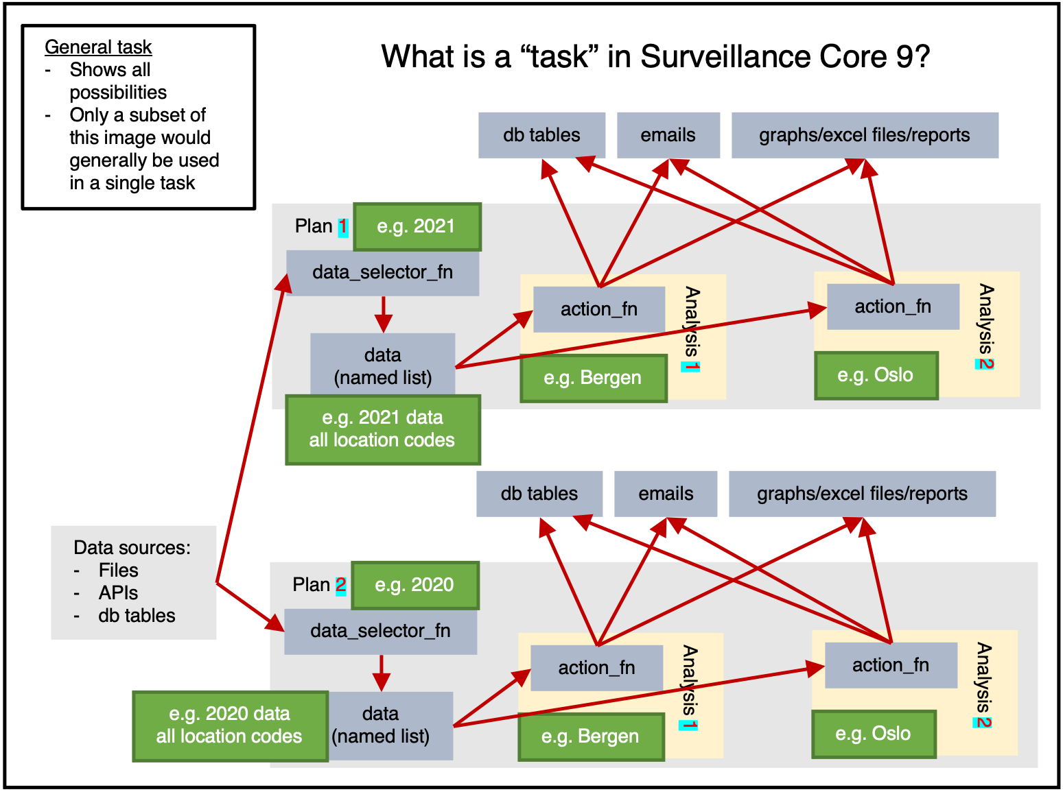
Figure 1 shows the available options within a task.
Data can be read from any source. Within a plan,
data_selector_fn extracts the data once (a
single data-pull). That data is then passed to each analysis, which
calls action_fn with:
- the extracted data
- the argset
- the tables
The action_fn can then:
- Write data or results to database tables
- Send emails
- Export graphs, Excel files, reports, or other files
A single task would typically do only a subset of these things.
Plan-heavy or analysis-heavy tasks?
A plan-heavy task has many plans with few analyses each. An analysis-heavy task has few plans with many analyses each.
Data-pulls are relatively slow, so fewer plans means less total time waiting for data. If each data-pull extracts a larger dataset, the analyses can subset it as needed (via argsets). Analysis-heavy tasks are therefore generally faster, at the cost of higher RAM usage.
If RAM is limited, use more plans with smaller data-pulls instead.
Figure 1 shows only 2 location-based
analyses. In practice, Norway had 356 municipalities in 2021. If
figure 1 had 2 plans (one for 2021 data, one for
2020 data) with 356 analyses each (one per location_code),
that would be an analysis-heavy approach.
Other vignettes
-
Installation and setup:
vignette("installation")covers database configuration and environment variables -
Package structure:
vignette("file-layout")explains how to organize your implementation files -
Creating tasks:
vignette("creating-a-task")walks through building your first surveillance task step by step
Example
The following example demonstrates the single-instance design
principle with weather data. Notice how the action function contains
only the logic that processes one location’s weather forecast. The same
function would scale across all Norwegian counties if you expanded the
for_each_plan. This is the same pattern NorSySS uses to
scale across 106 diseases and 378 locations.
The following example walks through designing and implementing a weather surveillance task.
Surveillance system setup
Start by creating a surveillance system. This object coordinates tables and tasks.
ss <- cs9::SurveillanceSystem_v9$new()Database table definition
As documented in more detail here, we create a database table for weather data and add it to the surveillance system.
ss$add_table(
  name_access = c("anon"),
  name_grouping = "example_weather",
  name_variant = NULL,
  field_types =  c(
    "granularity_time" = "TEXT",
    "granularity_geo" = "TEXT",
    "country_iso3" = "TEXT",
    "location_code" = "TEXT",
    "border" = "INTEGER",
    "age" = "TEXT",
    "sex" = "TEXT",

    "isoyear" = "INTEGER",
    "isoweek" = "INTEGER",
    "isoyearweek" = "TEXT",
    "season" = "TEXT",
    "seasonweek" = "DOUBLE",

    "calyear" = "INTEGER",
    "calmonth" = "INTEGER",
    "calyearmonth" = "TEXT",

    "date" = "DATE",

    "tg" = "DOUBLE",
    "tx" = "DOUBLE",
    "tn" = "DOUBLE"
  ),
  keys = c(
    "granularity_time",
    "location_code",
    "date",
    "age",
    "sex"
  ),
  validator_field_types = csdb::validator_field_types_csfmt_rts_data_v1,
  validator_field_contents = csdb::validator_field_contents_csfmt_rts_data_v1
)
Task configuration
Tasks are registered with ss$add_task:
# tm_run_task("example_weather_import_data_from_api")
ss$add_task(
  name_grouping = "example_weather",
  name_action = "import_data_from_api",
  name_variant = NULL,
  cores = 1,
  plan_analysis_fn_name = NULL, # "PACKAGE::TASK_NAME_plan_analysis"
  for_each_plan = plnr::expand_list(
    location_code = "county03" # fhidata::norway_locations_names()[granularity_geo %in% c("county")]$location_code
  ),
  for_each_analysis = NULL,
  universal_argset = NULL,
  upsert_at_end_of_each_plan = FALSE,
  insert_at_end_of_each_plan = FALSE,
  action_fn_name = "example_weather_import_data_from_api_action",
  data_selector_fn_name = "example_weather_import_data_from_api_data_selector",
  tables = list(
    # input

    # output
    "anon_example_weather" = ss$tables$anon_example_weather
  )
)
Several parameters are worth explaining in more detail.
for_each_plan
for_each_plan expects a list. Each element corresponds
to one plan; its values are added to the argset for every analysis
inside that plan.
The following code produces 4 plans with 1 analysis each, where each
analysis receives argset$var_1 and
argset$var_2:
for_each_plan <- list()
for_each_plan[[1]] <- list(
  var_1 = 1,
  var_2 = "a"
)
for_each_plan[[2]] <- list(
  var_1 = 2,
  var_2 = "b"
)
for_each_plan[[3]] <- list(
  var_1 = 1,
  var_2 = "a"
)
for_each_plan[[4]] <- list(
  var_1 = 2,
  var_2 = "b"
)
Every task needs at least 1 plan. The simplest plan possible is:
plnr::expand_list(
  x = 1
)
#> [[1]]
#> [[1]]$x
#> [1] 1
plnr::expand_list
plnr::expand_list works like expand.grid,
but returns a list instead of a data frame.
The four-element example above can be written more concisely:
for_each_plan <- plnr::expand_list(
  var_1 = c(1,2),
  var_2 = c("a", "b")
)
for_each_plan
#> [[1]]
#> [[1]]$var_1
#> [1] 1
#>
#> [[1]]$var_2
#> [1] "a"
#>
#>
#> [[2]]
#> [[2]]$var_1
#> [1] 2
#>
#> [[2]]$var_2
#> [1] "a"
#>
#>
#> [[3]]
#> [[3]]$var_1
#> [1] 1
#>
#> [[3]]$var_2
#> [1] "b"
#>
#>
#> [[4]]
#> [[4]]$var_1
#> [1] 2
#>
#> [[4]]$var_2
#> [1] "b"
for_each_analysis
for_each_plan generates
length(for_each_plan) plans. for_each_analysis
works the same way, but generates analyses within each
plan.
upsert_at_end_of_each_plan
When TRUE and tables contains a table named
output, the return value of action_fn is
upserted to tables$output at the end of each
plan.
When TRUE and action_fn returns a named
list, each element is upserted to the corresponding
tables$NAME_FROM_LIST at the end of each
plan.
If you upsert or insert manually from within action_fn,
you can only do so at the end of each analysis.
insert_at_end_of_each_plan
Same as upsert_at_end_of_each_plan, but inserts instead
of upserts.
If you insert manually from within action_fn, you can
only do so at the end of each analysis.
action_fn_name
A character string naming the action function, preferably including the package name.
data_selector_fn
The data_selector_fn extracts data for each plan.
The block inside if(plnr::is_run_directly()){ is for
interactive development. Running the function manually executes that
block, which loads argset and tables into your
environment so you can step through the rest of the code.
index_plan <- 1

argset <- ss$shortcut_get_argset("example_weather_import_data_from_api", index_plan = index_plan)
tables <- ss$shortcut_get_tables("example_weather_import_data_from_api")

print(argset)
#> $`**universal**`
#> [1] "*"
#>
#> $`**plan**`
#> [1] "*"
#>
#> $location_code
#> [1] "county03"
#>
#> $`**analysis**`
#> [1] "*"
#>
#> $`**automatic**`
#> [1] "*"
#>
#> $index
#> [1] 1
#>
#> $today
#> [1] "2025-08-21"
#>
#> $yesterday
#> [1] "2025-08-20"
#>
#> $index_plan
#> [1] 1
#>
#> $index_analysis
#> [1] 1
#>
#> $first_analysis
#> [1] TRUE
#>
#> $last_analysis
#> [1] TRUE
#>
#> $within_plan_first_analysis
#> [1] TRUE
#>
#> $within_plan_last_analysis
#> [1] TRUE
print(tables)
#> $anon_example_weather
#> public.anon_example_weather (disconnected)
#>
#>   1: granularity_time (TEXT) (KEY)
#>   2: granularity_geo (TEXT)
#>   3: country_iso3 (TEXT)
#>   4: location_code (TEXT) (KEY)
#>   5: border (INTEGER)
#>   6: age (TEXT) (KEY)
#>   7: sex (TEXT) (KEY)
#>   8: isoyear (INTEGER)
#>   9: isoweek (INTEGER)
#>  10: isoyearweek (TEXT)
#>  11: season (TEXT)
#>  12: seasonweek (DOUBLE)
#>  13: calyear (INTEGER)
#>  14: calmonth (INTEGER)
#>  15: calyearmonth (TEXT)
#>  16: date (DATE) (KEY)
#>  17: tg (DOUBLE)
#>  18: tx (DOUBLE)
#>  19: tn (DOUBLE)
#>  20: auto_last_updated_datetime (DATETIME)
# **** data_selector **** ----
#' example_weather_import_data_from_api (data selector)
#' @param argset Argset
#' @param tables DB tables
#' @export
example_weather_import_data_from_api_data_selector = function(argset, tables){
  if(plnr::is_run_directly()){
    # global$ss$shortcut_get_plans_argsets_as_dt("example_weather_import_data_from_api")

    index_plan <- 1

    argset <- ss$shortcut_get_argset("example_weather_import_data_from_api", index_plan = index_plan)
    tables <- ss$shortcut_get_tables("example_weather_import_data_from_api")
  }

  # find the mid lat/long for the specified location_code
  gps <- fhimaps::norway_nuts3_map_b2020_default_dt[location_code == argset$location_code,.(
    lat = mean(lat),
    long = mean(long)
  )]

  # download the forecast for the specified location_code
  d <- httr::GET(glue::glue("https://api.met.no/weatherapi/locationforecast/2.0/classic?lat={gps$lat}&lon={gps$long}"), httr::content_type_xml())
  d <- xml2::read_xml(d$content)

  # The variable returned must be a named list
  retval <- list(
    "data" = d
  )
  retval
}
action_fn
The if(plnr::is_run_directly()){ block works the same
way here: running the function manually loads data,
argset, and tables so you can work through the
analysis interactively.
index_plan <- 1
index_analysis <- 1

data <- ss$shortcut_get_data("example_weather_import_data_from_api", index_plan = index_plan)
argset <- ss$shortcut_get_argset("example_weather_import_data_from_api", index_plan = index_plan, index_analysis = index_analysis)
tables <- ss$shortcut_get_tables("example_weather_import_data_from_api")

print(data)
#> $data
#> {xml_document}
#> <weatherdata noNamespaceSchemaLocation="https://schema.api.met.no/schemas/weatherapi-0.4.xsd" created="2025-08-21T13:28:23Z" xmlns:xsi="http://www.w3.org/2001/XMLSchema-instance">
#> [1] <meta>\n  <model name="met_public_forecast" termin="2025-08-21T13:00:00Z" ...
#> [2] <product class="pointData">\n  <time datatype="forecast" from="2025-08-21 ...
#>
#> $hash
#> $hash$current
#> [1] "fa7c1fd90a6d9bf24040ae24919e6972"
#>
#> $hash$current_elements
#> $hash$current_elements$data
#> [1] "edf868d91cd1f5fe47b57b2aeb1d010d"
print(argset)
#> $`**universal**`
#> [1] "*"
#>
#> $`**plan**`
#> [1] "*"
#>
#> $location_code
#> [1] "county03"
#>
#> $`**analysis**`
#> [1] "*"
#>
#> $`**automatic**`
#> [1] "*"
#>
#> $index
#> [1] 1
#>
#> $today
#> [1] "2025-08-21"
#>
#> $yesterday
#> [1] "2025-08-20"
#>
#> $index_plan
#> [1] 1
#>
#> $index_analysis
#> [1] 1
#>
#> $first_analysis
#> [1] TRUE
#>
#> $last_analysis
#> [1] TRUE
#>
#> $within_plan_first_analysis
#> [1] TRUE
#>
#> $within_plan_last_analysis
#> [1] TRUE
print(tables)
#> $anon_example_weather
#> public.anon_example_weather (disconnected)
#>
#>   1: granularity_time (TEXT) (KEY)
#>   2: granularity_geo (TEXT)
#>   3: country_iso3 (TEXT)
#>   4: location_code (TEXT) (KEY)
#>   5: border (INTEGER)
#>   6: age (TEXT) (KEY)
#>   7: sex (TEXT) (KEY)
#>   8: isoyear (INTEGER)
#>   9: isoweek (INTEGER)
#>  10: isoyearweek (TEXT)
#>  11: season (TEXT)
#>  12: seasonweek (DOUBLE)
#>  13: calyear (INTEGER)
#>  14: calmonth (INTEGER)
#>  15: calyearmonth (TEXT)
#>  16: date (DATE) (KEY)
#>  17: tg (DOUBLE)
#>  18: tx (DOUBLE)
#>  19: tn (DOUBLE)
#>  20: auto_last_updated_datetime (DATETIME)
# **** action **** ----
#' example_weather_import_data_from_api (action)
#' @param data Data
#' @param argset Argset
#' @param tables DB tables
#' @export
example_weather_import_data_from_api_action <- function(data, argset, tables) {
  # tm_run_task("example_weather_import_data_from_api")

  if(plnr::is_run_directly()){
    # global$ss$shortcut_get_plans_argsets_as_dt("example_weather_import_data_from_api")

    index_plan <- 1
    index_analysis <- 1

    data <- ss$shortcut_get_data("example_weather_import_data_from_api", index_plan = index_plan)
    argset <- ss$shortcut_get_argset("example_weather_import_data_from_api", index_plan = index_plan, index_analysis = index_analysis)
    tables <- ss$shortcut_get_tables("example_weather_import_data_from_api")
  }

  # code goes here
  # special case that runs before everything
  if(argset$first_analysis == TRUE){

  }

  a <- data$data

  baz <- xml2::xml_find_all(a, ".//maxTemperature")
  res <- vector("list", length = length(baz))
  for (i in seq_along(baz)) {
    parent <- xml2::xml_parent(baz[[i]])
    grandparent <- xml2::xml_parent(parent)
    time_from <- xml2::xml_attr(grandparent, "from")
    time_to <- xml2::xml_attr(grandparent, "to")
    x <- xml2::xml_find_all(parent, ".//minTemperature")
    temp_min <- xml2::xml_attr(x, "value")
    x <- xml2::xml_find_all(parent, ".//maxTemperature")
    temp_max <- xml2::xml_attr(x, "value")
    res[[i]] <- data.frame(
      time_from = as.character(time_from),
      time_to = as.character(time_to),
      tx = as.numeric(temp_max),
      tn = as.numeric(temp_min)
    )
  }
  res <- rbindlist(res)
  res <- res[stringr::str_sub(time_from, 12, 13) %in% c("00", "06", "12", "18")]
  res[, date := as.Date(stringr::str_sub(time_from, 1, 10))]
  res[, N := .N, by = date]
  res <- res[N == 4]
  res <- res[
    ,
    .(
      tg = NA,
      tx = max(tx),
      tn = min(tn)
    ),
    keyby = .(date)
  ]

  # we look at the downloaded data
  print("Data after downloading")
  print(res)

  # we now need to format it
  res[, granularity_time := "day"]
  res[, sex := "total"]
  res[, age := "total"]
  res[, location_code := argset$location_code]
  res[, border := 2020]

  # fill in missing structural variables
  cstidy::set_csfmt_rts_data_v1(res)

  # we look at the downloaded data
  print("Data after missing structural variables filled in")
  print(res)

  # put data in db table
  # tables$TABLE_NAME$insert_data(d)
  tables$anon_example_weather$upsert_data(res)
  # tables$TABLE_NAME$drop_all_rows_and_then_upsert_data(d)

  # special case that runs after everything
  # copy to anon_web?
  if(argset$last_analysis == TRUE){
    # cs9::copy_into_new_table_where(
    #   table_from = "anon_X",
    #   table_to = "anon_web_X"
    # )
  }
}
Run the task
ss$run_task("example_weather_import_data_from_api")
#> task: example_weather_import_data_from_api
#> Running task=example_weather_import_data_from_api with plans=1 and analyses=1
#> plans=sequential, argset=sequential with cores=1
#>
#> [1] "Data after downloading"
#> Key: <date>
#>          date     tg    tx    tn
#>        <Date> <lgcl> <num> <num>
#> 1: 2025-08-22     NA  16.0   8.8
#> 2: 2025-08-23     NA  17.6   8.0
#> 3: 2025-08-24     NA  18.4   9.8
#> 4: 2025-08-25     NA  18.1   8.8
#> 5: 2025-08-26     NA  18.8   8.9
#> 6: 2025-08-27     NA  19.7   9.2
#> 7: 2025-08-28     NA  20.4  10.2
#> 8: 2025-08-29     NA  19.0  10.1
#> 9: 2025-08-30     NA  16.9  12.1
#> [1] "Data after missing structural variables filled in"
#>    granularity_time granularity_geo country_iso3 location_code border    age
#>              <char>          <char>       <char>        <char>  <int> <char>
#> 1:              day          county          nor      county03   2020  total
#> 2:              day          county          nor      county03   2020  total
#> 3:              day          county          nor      county03   2020  total
#> 4:              day          county          nor      county03   2020  total
#> 5:              day          county          nor      county03   2020  total
#> 6:              day          county          nor      county03   2020  total
#> 7:              day          county          nor      county03   2020  total
#> 8:              day          county          nor      county03   2020  total
#> 9:              day          county          nor      county03   2020  total
#>       sex isoyear isoweek isoyearweek season seasonweek calyear calmonth
#>    <char>   <int>   <int>      <char> <char>      <num>   <int>    <int>
#> 1:  total      NA      NA        <NA>   <NA>         NA      NA       NA
#> 2:  total      NA      NA        <NA>   <NA>         NA      NA       NA
#> 3:  total      NA      NA        <NA>   <NA>         NA      NA       NA
#> 4:  total      NA      NA        <NA>   <NA>         NA      NA       NA
#> 5:  total      NA      NA        <NA>   <NA>         NA      NA       NA
#> 6:  total      NA      NA        <NA>   <NA>         NA      NA       NA
#> 7:  total      NA      NA        <NA>   <NA>         NA      NA       NA
#> 8:  total      NA      NA        <NA>   <NA>         NA      NA       NA
#> 9:  total      NA      NA        <NA>   <NA>         NA      NA       NA
#>    calyearmonth       date     tg    tx    tn
#>          <char>     <Date> <lgcl> <num> <num>
#> 1:         <NA> 2025-08-22     NA  16.0   8.8
#> 2:         <NA> 2025-08-23     NA  17.6   8.0
#> 3:         <NA> 2025-08-24     NA  18.4   9.8
#> 4:         <NA> 2025-08-25     NA  18.1   8.8
#> 5:         <NA> 2025-08-26     NA  18.8   8.9
#> 6:         <NA> 2025-08-27     NA  19.7   9.2
#> 7:         <NA> 2025-08-28     NA  20.4  10.2
#> 8:         <NA> 2025-08-29     NA  19.0  10.1
#> 9:         <NA> 2025-08-30     NA  16.9  12.1
#> Error in super$upsert_data(newdata, drop_indexes, verbose): upsert_load_data_infile not validated in anon_example_weather. granularity_time
Common task patterns
Importing data
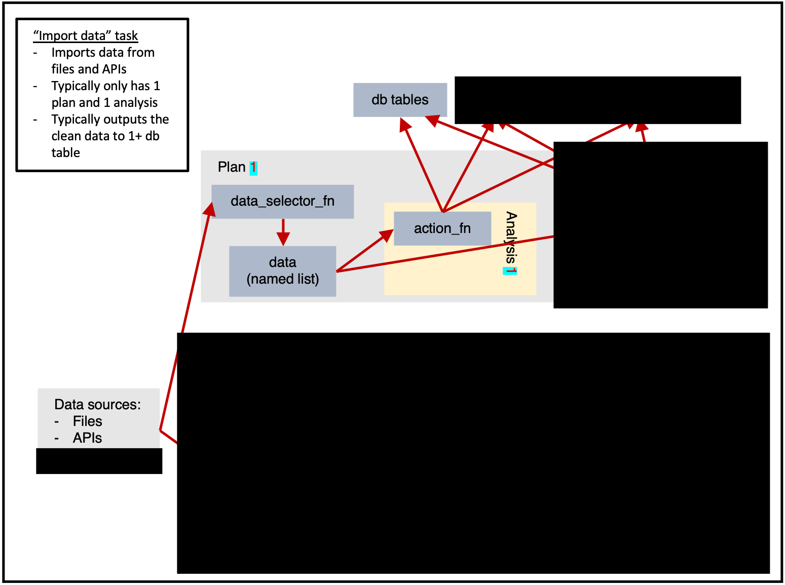
ss$add_task(
  name_grouping = "example",
  name_action = "import_data",
  name_variant = NULL,
  cores = 1,
  plan_analysis_fn_name = NULL,
  for_each_plan = plnr::expand_list(
    x = 1
  ),
  for_each_analysis = NULL,
  universal_argset = list(
    folder = cs9::path("input", "example")
  ),
  upsert_at_end_of_each_plan = FALSE,
  insert_at_end_of_each_plan = FALSE,
  action_fn_name = "example_import_data_action",
  data_selector_fn_name = "example_import_data_data_selector",
  tables = list(
    # input

    # output
    "output" = ss$tables$output
  )
)
Analysis
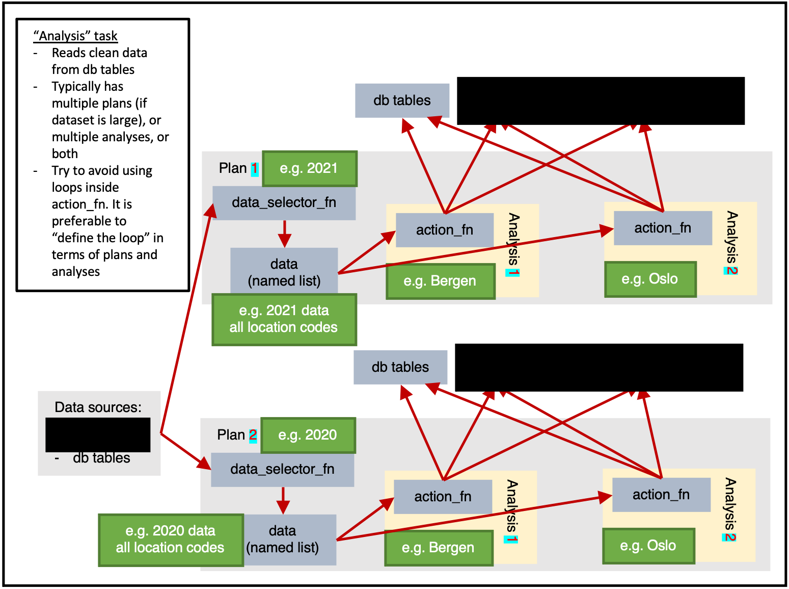
ss$add_task(
  name_grouping = "example",
  name_action = "analysis",
  name_variant = NULL,
  cores = 1,
  plan_analysis_fn_name = NULL,
  for_each_plan = plnr::expand_list(
    location_code = csdata::nor_locations_names()[granularity_geo %in% c("county")]$location_code
  ),
  for_each_analysis = NULL,
  universal_argset = NULL,
  upsert_at_end_of_each_plan = FALSE,
  insert_at_end_of_each_plan = FALSE,
  action_fn_name = "example_analysis_action",
  data_selector_fn_name = "example_analysis_data_selector",
  tables = list(
    # input
    "input" = ss$tables$input,

    # output
    "output" = ss$tables
  )
)
Exporting multiple sets of results
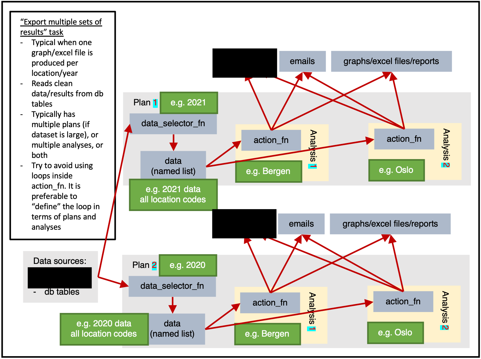
ss$add_task(
  name_grouping = "example",
  name_action = "export_results",
  name_variant = NULL,
  cores = 1,
  plan_analysis_fn_name = NULL,
  for_each_plan = plnr::expand_list(
    location_code = csdata::nor_locations_names()[granularity_geo %in% c("county")]$location_code
  ),
  for_each_analysis = NULL,
  universal_argset = list(
    folder = cs9::path("output", "example")
  ),
  upsert_at_end_of_each_plan = FALSE,
  insert_at_end_of_each_plan = FALSE,
  action_fn_name = "example_export_results_action",
  data_selector_fn_name = "example_export_results_data_selector",
  tables = list(
    # input
    "input" = ss$tables$input

    # output
  )
)
Exporting combined results
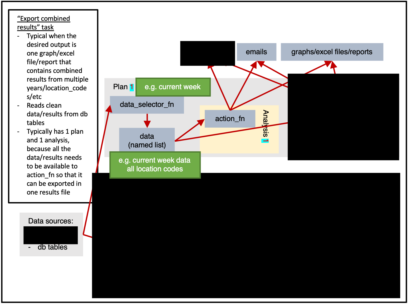
ss$tables(
  name_grouping = "example",
  name_action = "export_results",
  name_variant = NULL,
  cores = 1,
  plan_analysis_fn_name = NULL,
  for_each_plan = plnr::expand_list(
    x = 1
  ),
  for_each_analysis = NULL,
  universal_argset = list(
    folder = cs9::path("output", "example"),
    granularity_geos = c("nation", "county")
  ),
  upsert_at_end_of_each_plan = FALSE,
  insert_at_end_of_each_plan = FALSE,
  action_fn_name = "example_export_results_action",
  data_selector_fn_name = "example_export_results_data_selector",
  tables = list(
    # input
    "input" = ss$tables$input

    # output
  )
)
Deployment
A typical development-to-production cycle looks like this:
-
Development: Use
devtools::load_all()for interactive development -
Testing: Run individual tasks with
global$ss$run_task("task_name") - Production: Deploy in Docker containers with Airflow scheduling
- Monitoring: Track execution through the built-in logging tables
What the framework handles for you
- Structured logging, at the level of the individual analysis: execution time, data volume processed, and which disease-location-demographic combination threw an error.
- Database management: schema validation, partitioning by time period, and bulk operations over millions of rows. Partitioning holds query performance steady as history accumulates over years. Data selectors keep the database structure out of the analysis code.
- Parallel computation, at the framework level. You write sequential R code. The same code runs on a laptop with 4 cores during development and a server with 20 cores in production.
- Validation workflows: completeness, temporal consistency, and outputs against expected ranges.
Getting started
The recommended starting point is the cs9example repository, which provides a working surveillance system you can adapt:
- Clone the cs9example repository
- Do a global find/replace of
"cs9example"with your package name - Update the table definitions in
03_tables.Rfor your data - Update the task definitions in
04_tasks.Rfor your analyses - Implement your task functions following the same patterns
Next steps
- Installation — database and environment setup
- Creating a task — step-by-step task implementation
- File layout — how to organize your package files