Introduction

csmaps ships the geometry of Norway as plain data.table objects. You can draw choropleth maps with ggplot2 alone, without sf, GDAL, or any other geolibrary.

csmaps is part of the Core Surveillance family of R packages. It covers counties, municipalities, and Oslo’s city wards across four redistricting years (2017, 2019, 2020 and 2024).

What csmaps saves you

To draw a map in R you usually install a geolibrary stack first: sf, and under it GDAL, PROJ and GEOS. You then read a shapefile and convert it. csmaps skips all of that. The polygons are already parsed and already simplified, and they are stored as tables of longitude and latitude points. One library() call and you are drawing.

That is the reason the package exists. On a locked-down work machine, or in a container you want to keep small, csmaps is a plain R package with no system dependencies.

Choosing a dataset

csmaps is almost all data. It exports one function, annotate_oslo_nor_map_bxxxx_split_dt(); everything else is a dataset. The names follow a single pattern, so you can build the name you want instead of searching for it:

<area>_<content>_b<year>_<layout>_<type>

part	values
`area`	`nor_county`, `nor_municip`, `oslo_ward` (`nor_xxx` = not tied to one area)
`content`	`map` (the polygons), `position_geolabels` (one label point per region), `position_title_insert_oslo` (where to place the “Oslo” label on an inset map)
`b<year>`	`b2017`, `b2019`, `b2020`, `b2024` — the borders in force that year
`layout`	`default`, `insert_oslo`, `split`
`type`	`dt` (a `data.table`) or `sf` (an `sf` object)

So the 2024 municipality polygons, as a data.table, are nor_municip_map_b2024_default_dt. Not every combination exists; list them:

items <- utils::data(package = "csmaps")$results[, "Item"]
length(items)
#> [1] 51
head(sort(items), 3)
#> [1] "nor_county_map_b2017_default_dt"     "nor_county_map_b2017_default_sf"    
#> [3] "nor_county_map_b2017_insert_oslo_dt"

The three layouts

default — Norway drawn where it is.
insert_oslo — the default map, plus a copy of Oslo magnified about 11 times and placed in the blank area east of the mainland. Oslo is 0.45 degrees of longitude wide, too small to read at national scale.
split — the three northern counties (Nordland, Troms and Finnmark) move down beside southern Norway. This brings the northern edge of the map from 71.2 degrees north to 65.7. No other region moves. The county split map also carries the magnified Oslo copy. The municipality split map does not.

csmaps holds no Svalbard and no Jan Mayen, so no layout moves them.

Two limits worth knowing

sf objects exist for the default layout only. There is no split or insert_oslo sf dataset:

layout <- sub("_(dt|sf)$", "", sub("^.*_b[0-9]{4}_", "", items))
type <- sub("^.*_", "", items)
table(layout, type)
#>              type
#> layout        dt sf
#>   default     18  9
#>   insert_oslo 18  0
#>   split        6  0

The 2024 municipality maps hold 356 municipalities, where csdata lists 357. Haram (municip_nor1580) separated from Ålesund on 1 January 2024 but has no polygon here, so Haram is still drawn inside Ålesund (municip_nor1508):

codes <- csmaps::nor_municip_map_b2024_default_dt$location_code
length(unique(codes))
#> [1] 356
"municip_nor1580" %in% codes
#> [1] FALSE

How it fits with csdata

location_code carries csdata’s codes exactly — county_nor03, municip_nor0301, wardoslo_nor030101 — so you can join a map to a csdata table with no crosswalk. csmaps itself needs no cs* package: it imports only data.table, ggplot2 and utils.

For the split and inset maps in full, see the Layout vignette. To shade regions by your own numbers, see Customize your maps. For the sf datasets and leaflet, see Interactive maps.

Setup

Load csmaps alongside ggplot2 and data.table:

library(csmaps)
#> csmaps 2026.8.6
#> https://niphr.github.io/csmaps/
library(ggplot2)
library(data.table)
#> 
#> Attaching package: 'data.table'
#> The following object is masked from 'package:base':
#> 
#>     %notin%
library(magrittr)

A first map

Every map is a data.table of polygon coordinates, so you can hand it straight to geom_polygon(). Here is the municipality map for the 2024 borders:

pd <- copy(csmaps::nor_municip_map_b2024_default_dt)
q <- ggplot()
q <- q + geom_polygon(
  data = pd,
  aes(
    x = long,
    y = lat,
    group = group
  ),
  color="black",
  fill="white",
  linewidth = 0.2
)
q <- q + theme_void()
q <- q + coord_quickmap()
q <- q + labs(title = "Default layout")
q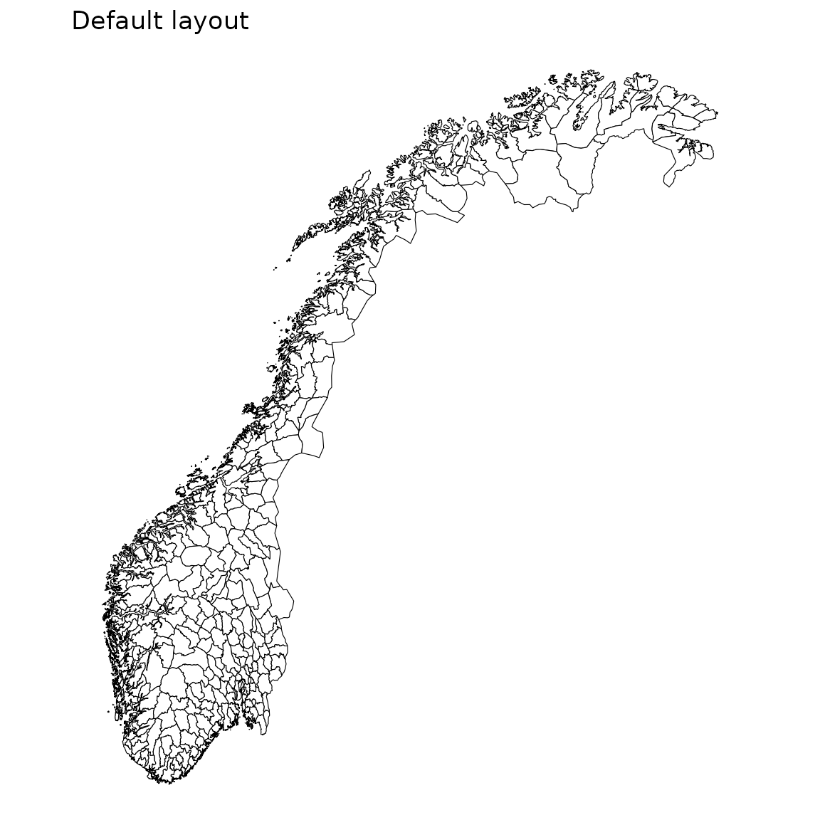

The same code draws the counties; only the dataset changes:

pd <- copy(csmaps::nor_county_map_b2024_default_dt)
q <- ggplot()
q <- q + geom_polygon(
  data = pd,
  aes(
    x = long,
    y = lat,
    group = group
  ),
  color="black",
  fill="white",
  linewidth = 0.4
)
q <- q + theme_void()
q <- q + coord_quickmap()
q <- q + labs(title = "Default layout")
q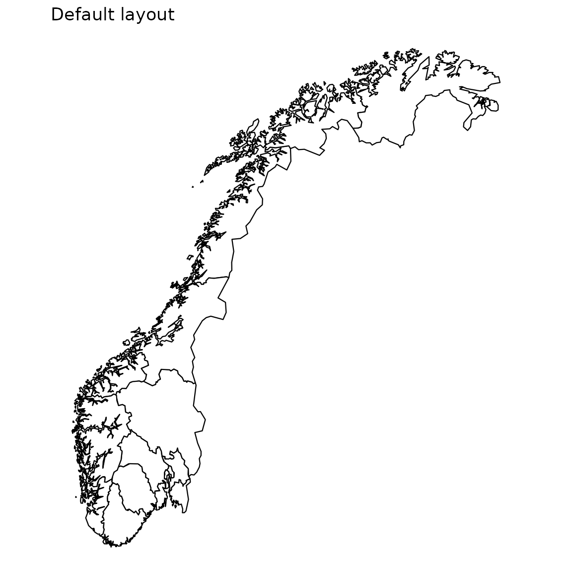

Where to next

For a split north/south view or an inset that enlarges Oslo, see the layout vignette. To shade regions by your own numbers, see customization. The full list of datasets lives in the reference.

Richard Aubrey White, Chi Zhang

2023-05-30