Split map of Norwegian counties in data.table format

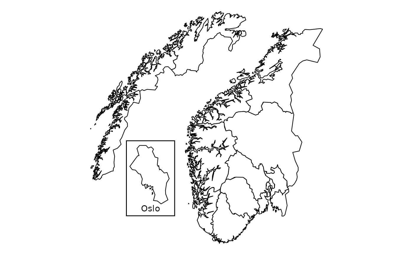
We package the map datasets for Norwegian counties, taken from Geonorge, so that you can draw them in ggplot2 with no geolibrary. The split layout moves the far-northern counties down beside southern Norway. This cuts the whitespace that a full-length map leaves. The layout also adds a magnified copy of Oslo in the lower left. This data is licensed under Creative Commons BY 4.0 (CC BY 4.0).

Returns two ggplot2::annotate() layers. The first is a white rectangle that spans longitude 0.5 to 3.9 and latitude 58.9 to 61.4. The second is the text "Oslo" at longitude 2.2, latitude 59.15. Those bounds enclose the magnified Oslo copy in nor_county_map_b2024_split_dt and nor_county_map_b2020_split_dt. Add the list to a ggplot2 plot with +, before the geom_polygon() that draws the map.

Usage

nor_county_map_b2024_split_dt

nor_county_map_b2020_split_dt

nor_county_position_geolabels_b2024_split_dt

nor_county_position_geolabels_b2020_split_dt

annotate_oslo_nor_map_bxxxx_split_dt()

Format

nor_county_map_b2024_split_dt and nor_county_map_b2020_split_dt are data.tables with one row per polygon vertex:

long: Longitude in decimal degrees (WGS84).
lat: Latitude in decimal degrees (WGS84).
order: Integer draw order carried over from the source polygon conversion. ggplot2::geom_polygon() follows row order, so you rarely need this column, and its values are not contiguous in every dataset.
group: Factor, one level per closed polygon ring; use as the group aesthetic in ggplot2. Several rings can share one location_code.
location_code: County code (e.g. "county_nor03").

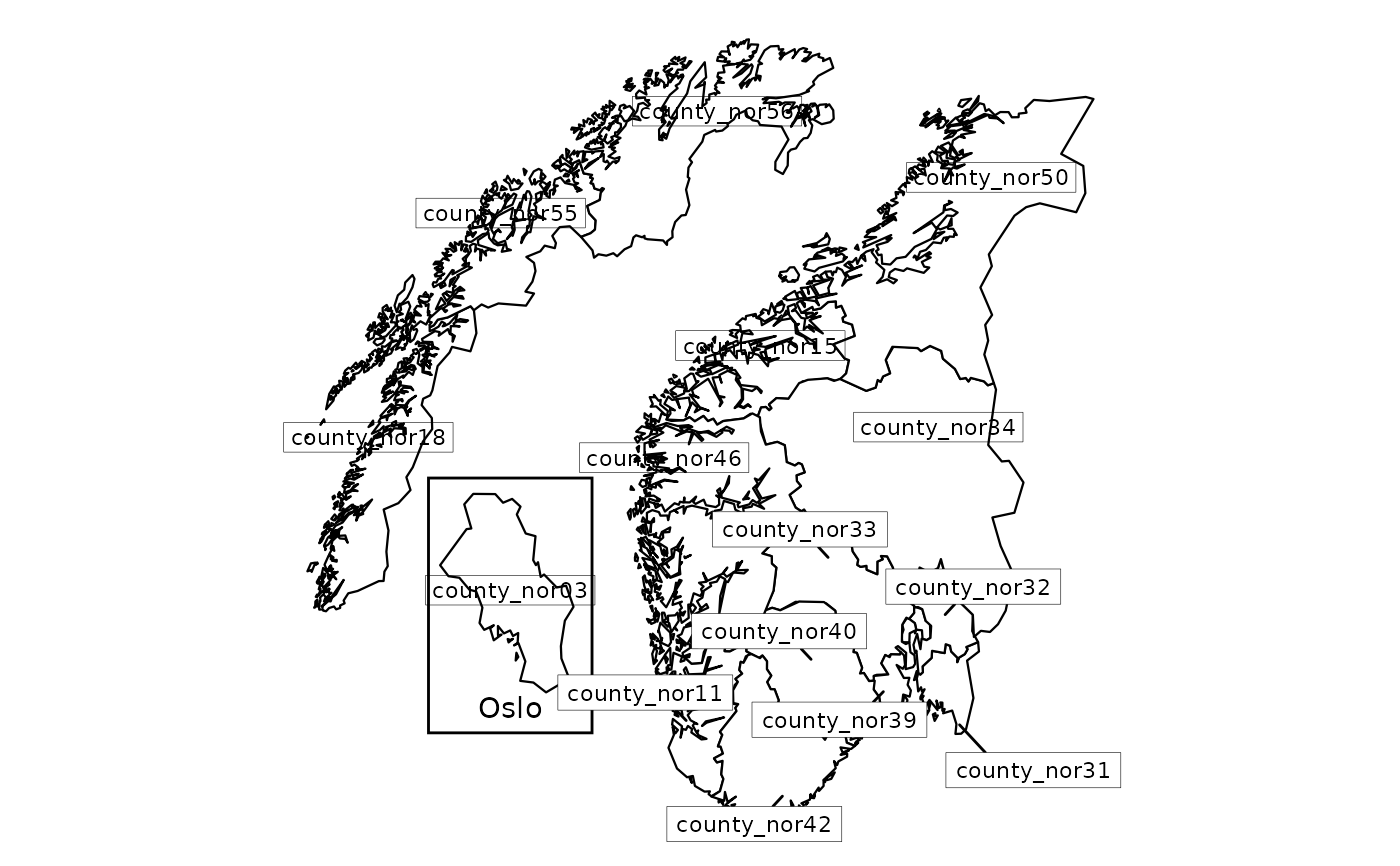
nor_county_position_geolabels_b2024_split_dt and nor_county_position_geolabels_b2020_split_dt are data.tables with one row per county:

location_code: County code (e.g. "county_nor03").
long: Longitude in decimal degrees (WGS84) of the label anchor.
lat: Latitude in decimal degrees (WGS84) of the label anchor.
repel: Logical layout flag. Draw the TRUE rows with ggrepel::geom_label_repel() and the FALSE rows with ggplot2::geom_label().

An object of class data.table (inherits from data.frame) with 4537 rows and 5 columns.

An object of class data.table (inherits from data.frame) with 15 rows and 4 columns.

An object of class data.table (inherits from data.frame) with 11 rows and 4 columns.

Source

Kartverket / Geonorge https://www.geonorge.no/. License: CC BY 4.0.

Value

A list of two ggplot2 layer objects (a rectangle and a text annotation). Add the list directly to a ggplot with +.

Details

Borders for 2024 (15 counties) and 2020 (11 counties) are provided. The 2024 layout moves Nordland (county_nor18), Troms (county_nor55) and Finnmark (county_nor56). The 2020 layout moves Nordland (county_nor18) and Troms og Finnmark (county_nor54). Every other county keeps its default coordinates. The package holds no Svalbard or Jan Mayen polygons, in this layout or any other.

Oslo appears twice. Both copies keep location_code == "county_nor03". The magnified copy takes group levels that start with "x". It spans longitude 0.74 to 3.52 and latitude 59.30 to 61.24. Draw a box and caption around it with annotate_oslo_nor_map_bxxxx_split_dt().

Each border year has a polygon table (nor_county_map_*) and a label table (nor_county_position_geolabels_*). The two hold the same set of location_code values, but different columns.

The municipality split maps carry no magnified Oslo copy, so this annotation draws an empty box on them.

Examples

# 2024 borders
library(ggplot2)
q <- ggplot(mapping = aes(x = long, y = lat))
q <- q + csmaps::annotate_oslo_nor_map_bxxxx_split_dt()
q <- q + geom_polygon(
  data = csmaps::nor_county_map_b2024_split_dt,
  mapping = aes(group = group),
  color = "black",
  fill = "white",
  linewidth = 0.4
)
q <- q + theme_void()
q <- q + coord_quickmap()
q


# 2024 borders
library(ggplot2)
q <- ggplot(mapping = aes(x = long, y = lat))
q <- q + csmaps::annotate_oslo_nor_map_bxxxx_split_dt()
q <- q + geom_polygon(
  data = csmaps::nor_county_map_b2024_split_dt,
  mapping = aes(group = group),
  color = "black",
  fill = "white",
  linewidth = 0.4
)
q <- q + ggrepel::geom_label_repel(
  data = csmaps::nor_county_position_geolabels_b2024_split_dt[repel==TRUE],
  mapping = aes(x = long, y = lat, label = location_code),
  size = 3,
  label.size = 0.1,
  label.r = grid::unit(0, "lines"),
  min.segment.length = 0
)
q <- q + geom_label(
  data = csmaps::nor_county_position_geolabels_b2024_split_dt[repel==FALSE],
  mapping = aes(x = long, y = lat, label = location_code),
  size = 3,
  label.size = 0.1,
  label.r = grid::unit(0, "lines")
)
#> Warning: The `label.size` argument of `geom_label()` is deprecated as of ggplot2 3.5.0.
#> ℹ Please use the `linewidth` argument instead.
q <- q + theme_void()
q <- q + coord_quickmap()
q


# 2020 borders
library(ggplot2)
q <- ggplot(mapping = aes(x = long, y = lat))
q <- q + csmaps::annotate_oslo_nor_map_bxxxx_split_dt()
q <- q + geom_polygon(
  data = csmaps::nor_county_map_b2020_split_dt,
  mapping = aes(group = group),
  color = "black",
  fill = "white",
  linewidth = 0.4
)
q <- q + theme_void()
q <- q + coord_quickmap()
q