Maps of Norwegian counties with an insert for Oslo in data.table format
Source:R/data_norway_county.R
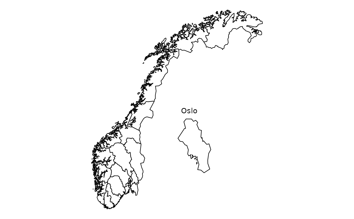
nor_county_map_bxxxx_insert_oslo_dt.RdWe package the map datasets for Norwegian counties, taken from Geonorge, so that you can draw them in ggplot2 with no geolibrary. Every county keeps its default position. The layout adds a magnified copy of Oslo in the blank area east of the mainland outline. This data is licensed under Creative Commons BY 4.0 (CC BY 4.0).
Usage
nor_county_map_b2024_insert_oslo_dt

nor_county_map_b2020_insert_oslo_dt

nor_county_map_b2019_insert_oslo_dt

nor_county_map_b2017_insert_oslo_dt

nor_county_position_geolabels_b2024_insert_oslo_dt

nor_county_position_geolabels_b2020_insert_oslo_dt

nor_county_position_geolabels_b2019_insert_oslo_dt

nor_county_position_geolabels_b2017_insert_oslo_dt
Format
The four nor_county_map_*_insert_oslo_dt datasets are
data.tables with one row per polygon vertex:
- long
Longitude in decimal degrees (WGS84).
- lat
Latitude in decimal degrees (WGS84).
- order
Integer draw order carried over from the source polygon conversion.
ggplot2::geom_polygon()follows row order, so you rarely need this column, and its values are not contiguous in every dataset.- group
Factor, one level per closed polygon ring; use as the
groupaesthetic in ggplot2. Several rings can share onelocation_code.- location_code
County code (e.g.
"county_nor03").
The four nor_county_position_geolabels_*_insert_oslo_dt datasets are
data.tables with one row per county:
- location_code
County code (e.g.
"county_nor03").- long
Longitude in decimal degrees (WGS84) of the label anchor.
- lat
Latitude in decimal degrees (WGS84) of the label anchor.
- repel
Logical layout flag. Draw the
TRUErows withggrepel::geom_label_repel()and theFALSErows withggplot2::geom_label().
An object of class data.table (inherits from data.frame) with 4537 rows and 5 columns.
An object of class data.table (inherits from data.frame) with 4780 rows and 5 columns.
An object of class data.table (inherits from data.frame) with 4589 rows and 5 columns.
An object of class data.table (inherits from data.frame) with 15 rows and 4 columns.
An object of class data.table (inherits from data.frame) with 11 rows and 4 columns.
An object of class data.table (inherits from data.frame) with 18 rows and 4 columns.
An object of class data.table (inherits from data.frame) with 19 rows and 4 columns.
Source
Kartverket / Geonorge https://www.geonorge.no/. License: CC BY 4.0.
Details
Borders for 2024, 2020, 2019, and 2017 are provided. The number of counties differs by border year: 15 in 2024, 11 in 2020, 18 in 2019, and 19 in 2017.
Oslo therefore appears twice. Both copies keep
location_code == "county_nor03". The magnified copy takes group
levels that start with "x". It spans longitude 17.99 to 23.08 and
latitude 60.39 to 63.96. Pair the dataset with
nor_xxx_position_title_insert_oslo_bxxxx_insert_oslo_dt, which
holds the coordinate for an "Oslo" caption above that copy.
Each border year has a polygon table (nor_county_map_*) and a label
table (nor_county_position_geolabels_*). The two hold the same set of
location_code values, but different columns.
See also
vignette("layout", package = "csmaps") draws
nor_county_map_b2024_insert_oslo_dt and explains the layout. No
vignette uses the 2020, 2019 or 2017 datasets, or any label dataset on this
page.
Other county maps:
nor_county_map_bxxxx_default_dt,
nor_county_map_bxxxx_default_sf,
nor_county_map_bxxxx_split_dt
Other insert-Oslo layout datasets:
nor_municip_map_bxxxx_insert_oslo_dt,
nor_xxx_position_title_insert_oslo_bxxxx_insert_oslo_dt
Examples
# 2024 borders
library(ggplot2)
q <- ggplot(mapping = aes(x = long, y = lat))
q <- q + geom_polygon(
data = csmaps::nor_county_map_b2024_insert_oslo_dt,
mapping = aes(group = group),
color = "black",
fill = "white",
linewidth = 0.4
)
q <- q + annotate(
"text",
x = csmaps::nor_xxx_position_title_insert_oslo_b2024_insert_oslo_dt$long,
y = csmaps::nor_xxx_position_title_insert_oslo_b2024_insert_oslo_dt$lat,
label = "Oslo"
)
q <- q + theme_void()
q <- q + coord_quickmap()
q
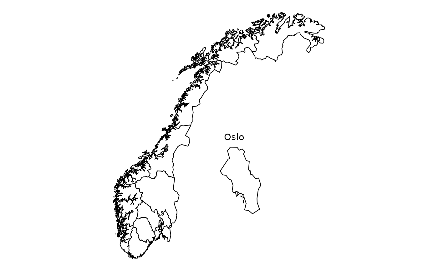 # 2020 borders
library(ggplot2)
q <- ggplot(mapping = aes(x = long, y = lat))
q <- q + geom_polygon(
data = csmaps::nor_county_map_b2020_insert_oslo_dt,
mapping = aes(group = group),
color = "black",
fill = "white",
linewidth = 0.4
)
q <- q + annotate(
"text",
x = csmaps::nor_xxx_position_title_insert_oslo_b2020_insert_oslo_dt$long,
y = csmaps::nor_xxx_position_title_insert_oslo_b2020_insert_oslo_dt$lat,
label = "Oslo"
)
q <- q + theme_void()
q <- q + coord_quickmap()
q
# 2020 borders
library(ggplot2)
q <- ggplot(mapping = aes(x = long, y = lat))
q <- q + geom_polygon(
data = csmaps::nor_county_map_b2020_insert_oslo_dt,
mapping = aes(group = group),
color = "black",
fill = "white",
linewidth = 0.4
)
q <- q + annotate(
"text",
x = csmaps::nor_xxx_position_title_insert_oslo_b2020_insert_oslo_dt$long,
y = csmaps::nor_xxx_position_title_insert_oslo_b2020_insert_oslo_dt$lat,
label = "Oslo"
)
q <- q + theme_void()
q <- q + coord_quickmap()
q
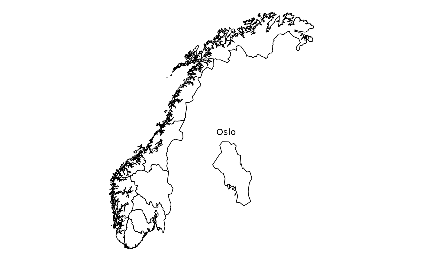 # 2019 borders
library(ggplot2)
q <- ggplot(mapping = aes(x = long, y = lat))
q <- q + geom_polygon(
data = csmaps::nor_county_map_b2019_insert_oslo_dt,
mapping = aes(group = group),
color = "black",
fill = "white",
linewidth = 0.4
)
q <- q + annotate(
"text",
x = csmaps::nor_xxx_position_title_insert_oslo_b2019_insert_oslo_dt$long,
y = csmaps::nor_xxx_position_title_insert_oslo_b2019_insert_oslo_dt$lat,
label = "Oslo"
)
q <- q + theme_void()
q <- q + coord_quickmap()
q
# 2019 borders
library(ggplot2)
q <- ggplot(mapping = aes(x = long, y = lat))
q <- q + geom_polygon(
data = csmaps::nor_county_map_b2019_insert_oslo_dt,
mapping = aes(group = group),
color = "black",
fill = "white",
linewidth = 0.4
)
q <- q + annotate(
"text",
x = csmaps::nor_xxx_position_title_insert_oslo_b2019_insert_oslo_dt$long,
y = csmaps::nor_xxx_position_title_insert_oslo_b2019_insert_oslo_dt$lat,
label = "Oslo"
)
q <- q + theme_void()
q <- q + coord_quickmap()
q
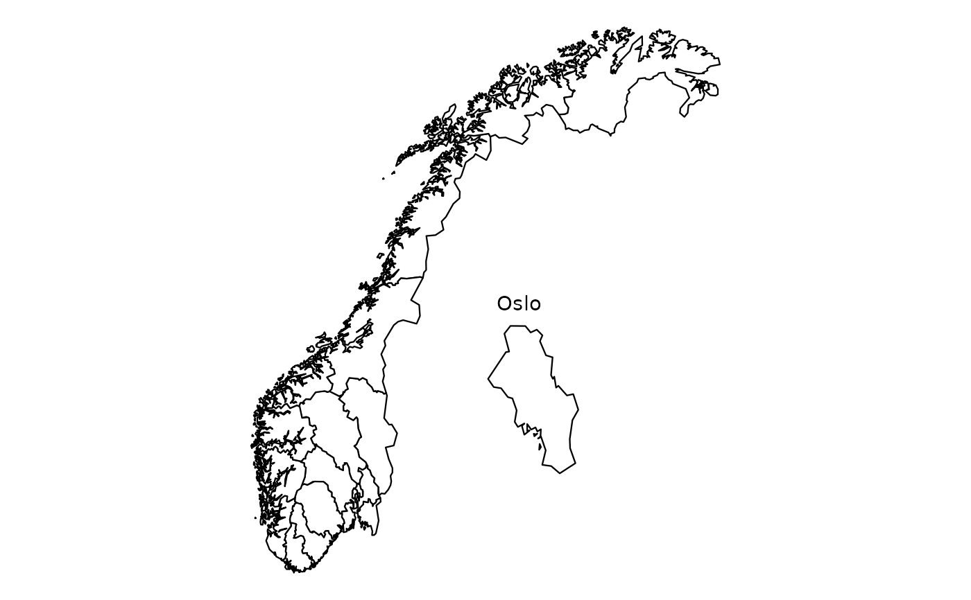 # 2017 borders
library(ggplot2)
q <- ggplot(mapping = aes(x = long, y = lat))
q <- q + geom_polygon(
data = csmaps::nor_county_map_b2017_insert_oslo_dt,
mapping = aes(group = group),
color = "black",
fill = "white",
linewidth = 0.4
)
q <- q + annotate(
"text",
x = csmaps::nor_xxx_position_title_insert_oslo_b2017_insert_oslo_dt$long,
y = csmaps::nor_xxx_position_title_insert_oslo_b2017_insert_oslo_dt$lat,
label = "Oslo"
)
q <- q + theme_void()
q <- q + coord_quickmap()
q
# 2017 borders
library(ggplot2)
q <- ggplot(mapping = aes(x = long, y = lat))
q <- q + geom_polygon(
data = csmaps::nor_county_map_b2017_insert_oslo_dt,
mapping = aes(group = group),
color = "black",
fill = "white",
linewidth = 0.4
)
q <- q + annotate(
"text",
x = csmaps::nor_xxx_position_title_insert_oslo_b2017_insert_oslo_dt$long,
y = csmaps::nor_xxx_position_title_insert_oslo_b2017_insert_oslo_dt$lat,
label = "Oslo"
)
q <- q + theme_void()
q <- q + coord_quickmap()
q