What cstidy is for
cstidy puts aggregated surveillance data into one standard shape: a
csfmt_rts_data table. You give it counts that already carry
a time column and a location column. It fills in the rest of the time
and geography columns that the shape requires, so everything downstream
can assume those columns are there.
cstidy does not turn individual records into counts. Aggregate first, then hand the result to cstidy.
Which format to use
Use csfmt_rts_data_v3, through
set_csfmt_rts_data_v3(). It is the current format and what
new work should target.
csfmt_rts_data_v1 and
csfmt_rts_data_v2 are deprecated. The mark is a
signpost, not an alarm. Neither format prints a deprecation warning, and
the mark changed no executable line, so nothing you have running will
break or start complaining. The rest of this page documents v2 and is
still accurate. Do not start there.
The three formats are siblings. None of them inherits from another.
d1 <- cstidy::generate_test_data()
d2 <- cstidy::generate_test_data()
d3 <- cstidy::generate_test_data()

cstidy::set_csfmt_rts_data_v1(d1)
cstidy::set_csfmt_rts_data_v2(d2)
cstidy::set_csfmt_rts_data_v3(d3)

class(d1)
#> [1] "csfmt_rts_data_v1" "data.table"        "data.frame"
class(d2)
#> [1] "csfmt_rts_data_v2" "data.table"        "data.frame"
class(d3)
#> [1] "csfmt_rts_data_v3" "data.table"        "data.frame"

inherits(d3, "csfmt_rts_data_v2")
#> [1] FALSE
Three things to know before you move to v3
v3 derives fewer columns, and removes none
Each format carries the list of columns it derives when the input lacks them. v2’s list holds 18 columns; v3’s holds 11.
Deriving is not removing. set_csfmt_rts_data_v3() takes
no column away, so a table built under v2 keeps every column it had.
What a move to v3 costs is the guarantee that those columns are present,
not the values in them.
length(attr(d2, "format_unified"))
#> [1] 18
length(attr(d3, "format_unified"))
#> [1] 11

d <- cstidy::generate_test_data()
cstidy::set_csfmt_rts_data_v2(d)
ncol(d)
#> [1] 19

# Take the old class off first. set_csfmt_rts_data_v3() on a table that is
# still csfmt_rts_data_v2 leaves it a csfmt_rts_data_v2.
cstidy::remove_class_csfmt_rts_data(d)
cstidy::set_csfmt_rts_data_v3(d)
ncol(d)
#> [1] 19
class(d)
#> [1] "csfmt_rts_data_v3" "data.table"        "data.frame"
v3 is weekly only
v3 fills in the time columns from isoyearweek and from
nothing else. Weekly data comes out complete.
A daily table keeps its date values and gets NA in every
other time column. Data that is not weekly stays on v2.
weekly <- data.table::data.table(
  isoyearweek = c("2020-34", "2020-35"),
  location_code = "nation_nor",
  deaths_n = c(1L, 2L)
)
cstidy::set_csfmt_rts_data_v3(weekly)
weekly[, .(isoyearweek, isoyear, isoweek, season, seasonweek, date)]
#>    isoyearweek isoyear isoweek    season seasonweek       date
#>         <char>   <int>   <int>    <char>      <num>     <Date>
#> 1:     2020-34    2020      34 2019/2020         52 2020-08-23
#> 2:     2020-35    2020      35 2020/2021          1 2020-08-30

daily <- data.table::data.table(
  granularity_time = "date",
  date = as.Date(c("2020-08-17", "2020-08-18")),
  location_code = "nation_nor",
  deaths_n = c(1L, 2L)
)
cstidy::set_csfmt_rts_data_v3(daily)
daily[, .(date, isoyear, isoweek, isoyearweek, season, seasonweek)]
#>          date isoyear isoweek isoyearweek season seasonweek
#>        <Date>   <int>   <int>      <char> <char>      <num>
#> 1: 2020-08-17      NA      NA        <NA>   <NA>         NA
#> 2: 2020-08-18      NA      NA        <NA>   <NA>         NA
csdb cannot check a v3 table, though it can store one
csdb ships table validators for
csfmt_rts_data_v1 and csfmt_rts_data_v2, and
nothing for v3, so a v3 column set fails both. That does not stop you
storing it. The validator is an ordinary argument to
csdb::DBTable_v9$new(): pass
validator_field_types_blank(), or a function of your own,
and the table writes. What you give up is the column check on the way
in, not the storage.
Where cstidy sits
cstidy imports csdata for Norwegian geography and
cstime for time conversions. It feeds csalert,
whose ens_collapse(heal = TRUE) returns a
csfmt_rts_data_v3.
Where to read next
-
vignette("csfmt_rts_data_v2", package = "cstidy")— the column-by-column reference for v2. -
vignette("benchmarks", package = "cstidy")— timings. -
?set_csfmt_rts_data_v3— the v3 reference. No vignette covers v3 yet.
Everything below documents csfmt_rts_data_v2.
csfmt_rts_data_v2
csfmt_rts_data_v2
(vignette("csfmt_rts_data_v2", package = "cstidy")) is the
Core Surveillance data format for real-time surveillance of infectious
diseases.
d <- cstidy::generate_test_data()
cstidy::set_csfmt_rts_data_v2(d)

# Looking at the dataset
d[]
#>     granularity_time granularity_geo country_iso3 location_code border     age
#>               <char>          <char>       <char>        <char>  <int>  <char>
#>  1:      isoyearweek          county          nor  county_nor42     NA    <NA>
#>  2:      isoyearweek          county          nor  county_nor32     NA    <NA>
#>  3:      isoyearweek          county          nor  county_nor33     NA    <NA>
#>  4:      isoyearweek          county          nor  county_nor56     NA    <NA>
#>  5:      isoyearweek          county          nor  county_nor34     NA    <NA>
#>  6:      isoyearweek          county          nor  county_nor15     NA    <NA>
#>  7:      isoyearweek          county          nor  county_nor18     NA    <NA>
#>  8:      isoyearweek          county          nor  county_nor03     NA    <NA>
#>  9:      isoyearweek          county          nor  county_nor11     NA    <NA>
#> 10:      isoyearweek          county          nor  county_nor40     NA    <NA>
#> 11:      isoyearweek          county          nor  county_nor55     NA    <NA>
#> 12:      isoyearweek          county          nor  county_nor50     NA    <NA>
#> 13:      isoyearweek          county          nor  county_nor39     NA    <NA>
#> 14:      isoyearweek          county          nor  county_nor46     NA    <NA>
#> 15:      isoyearweek          county          nor  county_nor31     NA    <NA>
#> 16:      isoyearweek          county          nor  county_nor42     NA   total
#> 17:      isoyearweek          county          nor  county_nor32     NA   total
#> 18:      isoyearweek          county          nor  county_nor33     NA   total
#> 19:      isoyearweek          county          nor  county_nor56     NA   total
#> 20:      isoyearweek          county          nor  county_nor34     NA   total
#> 21:      isoyearweek          county          nor  county_nor15     NA   total
#> 22:      isoyearweek          county          nor  county_nor18     NA   total
#> 23:      isoyearweek          county          nor  county_nor03     NA   total
#> 24:      isoyearweek          county          nor  county_nor11     NA   total
#> 25:      isoyearweek          county          nor  county_nor40     NA   total
#> 26:      isoyearweek          county          nor  county_nor55     NA   total
#> 27:      isoyearweek          county          nor  county_nor50     NA   total
#> 28:      isoyearweek          county          nor  county_nor39     NA   total
#> 29:      isoyearweek          county          nor  county_nor46     NA   total
#> 30:      isoyearweek          county          nor  county_nor31     NA   total
#> 31:      isoyearweek          county          nor  county_nor42     NA 000_005
#> 32:      isoyearweek          county          nor  county_nor32     NA 000_005
#> 33:      isoyearweek          county          nor  county_nor33     NA 000_005
#> 34:      isoyearweek          county          nor  county_nor56     NA 000_005
#> 35:      isoyearweek          county          nor  county_nor34     NA 000_005
#> 36:      isoyearweek          county          nor  county_nor15     NA 000_005
#> 37:      isoyearweek          county          nor  county_nor18     NA 000_005
#> 38:      isoyearweek          county          nor  county_nor03     NA 000_005
#> 39:      isoyearweek          county          nor  county_nor11     NA 000_005
#> 40:      isoyearweek          county          nor  county_nor40     NA 000_005
#> 41:      isoyearweek          county          nor  county_nor55     NA 000_005
#> 42:      isoyearweek          county          nor  county_nor50     NA 000_005
#> 43:      isoyearweek          county          nor  county_nor39     NA 000_005
#> 44:      isoyearweek          county          nor  county_nor46     NA 000_005
#> 45:      isoyearweek          county          nor  county_nor31     NA 000_005
#>     granularity_time granularity_geo country_iso3 location_code border     age
#>               <char>          <char>       <char>        <char>  <int>  <char>
#>        sex isoyear isoweek isoyearweek isoquarter isoyearquarter    season
#>     <char>   <int>   <int>      <char>      <int>         <char>    <char>
#>  1:   <NA>    2022       3     2022-03          1        2022-Q1 2021/2022
#>  2:   <NA>    2022       3     2022-03          1        2022-Q1 2021/2022
#>  3:   <NA>    2022       3     2022-03          1        2022-Q1 2021/2022
#>  4:   <NA>    2022       3     2022-03          1        2022-Q1 2021/2022
#>  5:   <NA>    2022       3     2022-03          1        2022-Q1 2021/2022
#>  6:   <NA>    2022       3     2022-03          1        2022-Q1 2021/2022
#>  7:   <NA>    2022       3     2022-03          1        2022-Q1 2021/2022
#>  8:   <NA>    2022       3     2022-03          1        2022-Q1 2021/2022
#>  9:   <NA>    2022       3     2022-03          1        2022-Q1 2021/2022
#> 10:   <NA>    2022       3     2022-03          1        2022-Q1 2021/2022
#> 11:   <NA>    2022       3     2022-03          1        2022-Q1 2021/2022
#> 12:   <NA>    2022       3     2022-03          1        2022-Q1 2021/2022
#> 13:   <NA>    2022       3     2022-03          1        2022-Q1 2021/2022
#> 14:   <NA>    2022       3     2022-03          1        2022-Q1 2021/2022
#> 15:   <NA>    2022       3     2022-03          1        2022-Q1 2021/2022
#> 16:  total    2022       3     2022-03          1        2022-Q1 2021/2022
#> 17:  total    2022       3     2022-03          1        2022-Q1 2021/2022
#> 18:  total    2022       3     2022-03          1        2022-Q1 2021/2022
#> 19:  total    2022       3     2022-03          1        2022-Q1 2021/2022
#> 20:  total    2022       3     2022-03          1        2022-Q1 2021/2022
#> 21:  total    2022       3     2022-03          1        2022-Q1 2021/2022
#> 22:  total    2022       3     2022-03          1        2022-Q1 2021/2022
#> 23:  total    2022       3     2022-03          1        2022-Q1 2021/2022
#> 24:  total    2022       3     2022-03          1        2022-Q1 2021/2022
#> 25:  total    2022       3     2022-03          1        2022-Q1 2021/2022
#> 26:  total    2022       3     2022-03          1        2022-Q1 2021/2022
#> 27:  total    2022       3     2022-03          1        2022-Q1 2021/2022
#> 28:  total    2022       3     2022-03          1        2022-Q1 2021/2022
#> 29:  total    2022       3     2022-03          1        2022-Q1 2021/2022
#> 30:  total    2022       3     2022-03          1        2022-Q1 2021/2022
#> 31:  total    2022       3     2022-03          1        2022-Q1 2021/2022
#> 32:  total    2022       3     2022-03          1        2022-Q1 2021/2022
#> 33:  total    2022       3     2022-03          1        2022-Q1 2021/2022
#> 34:  total    2022       3     2022-03          1        2022-Q1 2021/2022
#> 35:  total    2022       3     2022-03          1        2022-Q1 2021/2022
#> 36:  total    2022       3     2022-03          1        2022-Q1 2021/2022
#> 37:  total    2022       3     2022-03          1        2022-Q1 2021/2022
#> 38:  total    2022       3     2022-03          1        2022-Q1 2021/2022
#> 39:  total    2022       3     2022-03          1        2022-Q1 2021/2022
#> 40:  total    2022       3     2022-03          1        2022-Q1 2021/2022
#> 41:  total    2022       3     2022-03          1        2022-Q1 2021/2022
#> 42:  total    2022       3     2022-03          1        2022-Q1 2021/2022
#> 43:  total    2022       3     2022-03          1        2022-Q1 2021/2022
#> 44:  total    2022       3     2022-03          1        2022-Q1 2021/2022
#> 45:  total    2022       3     2022-03          1        2022-Q1 2021/2022
#>        sex isoyear isoweek isoyearweek isoquarter isoyearquarter    season
#>     <char>   <int>   <int>      <char>      <int>         <char>    <char>
#>     seasonweek calyear calmonth calyearmonth       date deaths_n
#>          <num>   <int>    <int>       <char>     <Date>    <int>
#>  1:         21      NA       NA         <NA> 2022-01-23        7
#>  2:         21      NA       NA         <NA> 2022-01-23        4
#>  3:         21      NA       NA         <NA> 2022-01-23        5
#>  4:         21      NA       NA         <NA> 2022-01-23        4
#>  5:         21      NA       NA         <NA> 2022-01-23        5
#>  6:         21      NA       NA         <NA> 2022-01-23        3
#>  7:         21      NA       NA         <NA> 2022-01-23        9
#>  8:         21      NA       NA         <NA> 2022-01-23        5
#>  9:         21      NA       NA         <NA> 2022-01-23        5
#> 10:         21      NA       NA         <NA> 2022-01-23        4
#> 11:         21      NA       NA         <NA> 2022-01-23        5
#> 12:         21      NA       NA         <NA> 2022-01-23        4
#> 13:         21      NA       NA         <NA> 2022-01-23        1
#> 14:         21      NA       NA         <NA> 2022-01-23        5
#> 15:         21      NA       NA         <NA> 2022-01-23        4
#> 16:         21      NA       NA         <NA> 2022-01-23        7
#> 17:         21      NA       NA         <NA> 2022-01-23        4
#> 18:         21      NA       NA         <NA> 2022-01-23        5
#> 19:         21      NA       NA         <NA> 2022-01-23        4
#> 20:         21      NA       NA         <NA> 2022-01-23        5
#> 21:         21      NA       NA         <NA> 2022-01-23        3
#> 22:         21      NA       NA         <NA> 2022-01-23        9
#> 23:         21      NA       NA         <NA> 2022-01-23        5
#> 24:         21      NA       NA         <NA> 2022-01-23        5
#> 25:         21      NA       NA         <NA> 2022-01-23        4
#> 26:         21      NA       NA         <NA> 2022-01-23        5
#> 27:         21      NA       NA         <NA> 2022-01-23        4
#> 28:         21      NA       NA         <NA> 2022-01-23        1
#> 29:         21      NA       NA         <NA> 2022-01-23        5
#> 30:         21      NA       NA         <NA> 2022-01-23        4
#> 31:         21      NA       NA         <NA> 2022-01-23        7
#> 32:         21      NA       NA         <NA> 2022-01-23        4
#> 33:         21      NA       NA         <NA> 2022-01-23        5
#> 34:         21      NA       NA         <NA> 2022-01-23        4
#> 35:         21      NA       NA         <NA> 2022-01-23        5
#> 36:         21      NA       NA         <NA> 2022-01-23        3
#> 37:         21      NA       NA         <NA> 2022-01-23        9
#> 38:         21      NA       NA         <NA> 2022-01-23        5
#> 39:         21      NA       NA         <NA> 2022-01-23        5
#> 40:         21      NA       NA         <NA> 2022-01-23        4
#> 41:         21      NA       NA         <NA> 2022-01-23        5
#> 42:         21      NA       NA         <NA> 2022-01-23        4
#> 43:         21      NA       NA         <NA> 2022-01-23        1
#> 44:         21      NA       NA         <NA> 2022-01-23        5
#> 45:         21      NA       NA         <NA> 2022-01-23        4
#>     seasonweek calyear calmonth calyearmonth       date deaths_n
#>          <num>   <int>    <int>       <char>     <Date>    <int>
Smart assignment
csfmt_rts_data_v2 supports smart assignment for time and
geography. When the bold variables below are set with
:=, the associated variables are automatically derived.
location_code:
- granularity_geo
- country_iso3
isoyear:
- granularity_time
- isoweek
- isoyearweek
- season
- seasonweek
- calyear
- calmonth
- calyearmonth
- date
isoyearweek:
- granularity_time
- isoyear
- isoweek
- season
- seasonweek
- calyear
- calmonth
- calyearmonth
- date
date:
- granularity_time
- isoyear
- isoweek
- isoyearweek
- season
- seasonweek
- calyear
- calmonth
- calyearmonth
d <- cstidy::generate_test_data()[1:5]
cstidy::set_csfmt_rts_data_v2(d)

# Looking at the dataset
d[]
#>    granularity_time granularity_geo country_iso3 location_code border    age
#>              <char>          <char>       <char>        <char>  <int> <char>
#> 1:      isoyearweek          county          nor  county_nor42     NA   <NA>
#> 2:      isoyearweek          county          nor  county_nor32     NA   <NA>
#> 3:      isoyearweek          county          nor  county_nor33     NA   <NA>
#> 4:      isoyearweek          county          nor  county_nor56     NA   <NA>
#> 5:      isoyearweek          county          nor  county_nor34     NA   <NA>
#>       sex isoyear isoweek isoyearweek isoquarter isoyearquarter    season
#>    <char>   <int>   <int>      <char>      <int>         <char>    <char>
#> 1:   <NA>    2022       3     2022-03          1        2022-Q1 2021/2022
#> 2:   <NA>    2022       3     2022-03          1        2022-Q1 2021/2022
#> 3:   <NA>    2022       3     2022-03          1        2022-Q1 2021/2022
#> 4:   <NA>    2022       3     2022-03          1        2022-Q1 2021/2022
#> 5:   <NA>    2022       3     2022-03          1        2022-Q1 2021/2022
#>    seasonweek calyear calmonth calyearmonth       date deaths_n
#>         <num>   <int>    <int>       <char>     <Date>    <int>
#> 1:         21      NA       NA         <NA> 2022-01-23        1
#> 2:         21      NA       NA         <NA> 2022-01-23        4
#> 3:         21      NA       NA         <NA> 2022-01-23        5
#> 4:         21      NA       NA         <NA> 2022-01-23        7
#> 5:         21      NA       NA         <NA> 2022-01-23        4

# Smart assignment of time columns (note how granularity_time, isoyear, isoyearweek, date all change)
d[1,isoyearweek := "2021-01"]
d
#>    granularity_time granularity_geo country_iso3 location_code border    age
#>              <char>          <char>       <char>        <char>  <int> <char>
#> 1:      isoyearweek          county          nor  county_nor42     NA   <NA>
#> 2:      isoyearweek          county          nor  county_nor32     NA   <NA>
#> 3:      isoyearweek          county          nor  county_nor33     NA   <NA>
#> 4:      isoyearweek          county          nor  county_nor56     NA   <NA>
#> 5:      isoyearweek          county          nor  county_nor34     NA   <NA>
#>       sex isoyear isoweek isoyearweek isoquarter isoyearquarter    season
#>    <char>   <int>   <int>      <char>      <int>         <char>    <char>
#> 1:   <NA>    2021       1     2021-01          1        2021-Q1 2020/2021
#> 2:   <NA>    2022       3     2022-03          1        2022-Q1 2021/2022
#> 3:   <NA>    2022       3     2022-03          1        2022-Q1 2021/2022
#> 4:   <NA>    2022       3     2022-03          1        2022-Q1 2021/2022
#> 5:   <NA>    2022       3     2022-03          1        2022-Q1 2021/2022
#>    seasonweek calyear calmonth calyearmonth       date deaths_n
#>         <num>   <int>    <int>       <char>     <Date>    <int>
#> 1:         19      NA       NA         <NA> 2021-01-10        1
#> 2:         21      NA       NA         <NA> 2022-01-23        4
#> 3:         21      NA       NA         <NA> 2022-01-23        5
#> 4:         21      NA       NA         <NA> 2022-01-23        7
#> 5:         21      NA       NA         <NA> 2022-01-23        4

# Smart assignment of time columns (note how granularity_time, isoyear, isoyearweek, date all change)
d[2,isoyear := 2019]
d
#>    granularity_time granularity_geo country_iso3 location_code border    age
#>              <char>          <char>       <char>        <char>  <int> <char>
#> 1:      isoyearweek          county          nor  county_nor42     NA   <NA>
#> 2:          isoyear          county          nor  county_nor32     NA   <NA>
#> 3:      isoyearweek          county          nor  county_nor33     NA   <NA>
#> 4:      isoyearweek          county          nor  county_nor56     NA   <NA>
#> 5:      isoyearweek          county          nor  county_nor34     NA   <NA>
#>       sex isoyear isoweek isoyearweek isoquarter isoyearquarter    season
#>    <char>   <int>   <int>      <char>      <int>         <char>    <char>
#> 1:   <NA>    2021       1     2021-01          1        2021-Q1 2020/2021
#> 2:   <NA>    2019      52     2019-52          1        2022-Q1      <NA>
#> 3:   <NA>    2022       3     2022-03          1        2022-Q1 2021/2022
#> 4:   <NA>    2022       3     2022-03          1        2022-Q1 2021/2022
#> 5:   <NA>    2022       3     2022-03          1        2022-Q1 2021/2022
#>    seasonweek calyear calmonth calyearmonth       date deaths_n
#>         <num>   <int>    <int>       <char>     <Date>    <int>
#> 1:         19      NA       NA         <NA> 2021-01-10        1
#> 2:         NA      NA       NA         <NA> 2019-12-29        4
#> 3:         21      NA       NA         <NA> 2022-01-23        5
#> 4:         21      NA       NA         <NA> 2022-01-23        7
#> 5:         21      NA       NA         <NA> 2022-01-23        4

# Smart assignment of time columns (note how granularity_time, isoyear, isoyearweek, date all change)
d[4:5,date := as.Date("2020-01-01")]
d
#>    granularity_time granularity_geo country_iso3 location_code border    age
#>              <char>          <char>       <char>        <char>  <int> <char>
#> 1:      isoyearweek          county          nor  county_nor42     NA   <NA>
#> 2:          isoyear          county          nor  county_nor32     NA   <NA>
#> 3:      isoyearweek          county          nor  county_nor33     NA   <NA>
#> 4:             date          county          nor  county_nor56     NA   <NA>
#> 5:             date          county          nor  county_nor34     NA   <NA>
#>       sex isoyear isoweek isoyearweek isoquarter isoyearquarter    season
#>    <char>   <int>   <int>      <char>      <int>         <char>    <char>
#> 1:   <NA>    2021       1     2021-01          1        2021-Q1 2020/2021
#> 2:   <NA>    2019      52     2019-52          1        2022-Q1      <NA>
#> 3:   <NA>    2022       3     2022-03          1        2022-Q1 2021/2022
#> 4:   <NA>    2020       1     2020-01          1        2020-Q1 2019/2020
#> 5:   <NA>    2020       1     2020-01          1        2020-Q1 2019/2020
#>    seasonweek calyear calmonth calyearmonth       date deaths_n
#>         <num>   <int>    <int>       <char>     <Date>    <int>
#> 1:         19      NA       NA         <NA> 2021-01-10        1
#> 2:         NA      NA       NA         <NA> 2019-12-29        4
#> 3:         21      NA       NA         <NA> 2022-01-23        5
#> 4:         19    2020        1     2020-M01 2020-01-01        7
#> 5:         19    2020        1     2020-M01 2020-01-01        4

# Smart assignment fails when multiple time columns are set
d[1,c("isoyear","isoyearweek") := .(2021,"2021-01")]
#> Warning in `[.csfmt_rts_data_v2`(d, 1, `:=`(c("isoyear", "isoyearweek"), :
#> Multiple time variables specified. Smart-assignment disabled.
d
#>    granularity_time granularity_geo country_iso3 location_code border    age
#>              <char>          <char>       <char>        <char>  <int> <char>
#> 1:      isoyearweek          county          nor  county_nor42     NA   <NA>
#> 2:          isoyear          county          nor  county_nor32     NA   <NA>
#> 3:      isoyearweek          county          nor  county_nor33     NA   <NA>
#> 4:             date          county          nor  county_nor56     NA   <NA>
#> 5:             date          county          nor  county_nor34     NA   <NA>
#>       sex isoyear isoweek isoyearweek isoquarter isoyearquarter    season
#>    <char>   <int>   <int>      <char>      <int>         <char>    <char>
#> 1:   <NA>    2021       1     2021-01          1        2021-Q1 2020/2021
#> 2:   <NA>    2019      52     2019-52          1        2022-Q1      <NA>
#> 3:   <NA>    2022       3     2022-03          1        2022-Q1 2021/2022
#> 4:   <NA>    2020       1     2020-01          1        2020-Q1 2019/2020
#> 5:   <NA>    2020       1     2020-01          1        2020-Q1 2019/2020
#>    seasonweek calyear calmonth calyearmonth       date deaths_n
#>         <num>   <int>    <int>       <char>     <Date>    <int>
#> 1:         19      NA       NA         <NA> 2021-01-10        1
#> 2:         NA      NA       NA         <NA> 2019-12-29        4
#> 3:         21      NA       NA         <NA> 2022-01-23        5
#> 4:         19    2020        1     2020-M01 2020-01-01        7
#> 5:         19    2020        1     2020-M01 2020-01-01        4

# Smart assignment of geo columns
d[1,c("location_code") := .("norge")]
d
#>    granularity_time granularity_geo country_iso3 location_code border    age
#>              <char>          <char>       <char>        <char>  <int> <char>
#> 1:      isoyearweek          nation          nor         norge     NA   <NA>
#> 2:          isoyear          county          nor  county_nor32     NA   <NA>
#> 3:      isoyearweek          county          nor  county_nor33     NA   <NA>
#> 4:             date          county          nor  county_nor56     NA   <NA>
#> 5:             date          county          nor  county_nor34     NA   <NA>
#>       sex isoyear isoweek isoyearweek isoquarter isoyearquarter    season
#>    <char>   <int>   <int>      <char>      <int>         <char>    <char>
#> 1:   <NA>    2021       1     2021-01          1        2021-Q1 2020/2021
#> 2:   <NA>    2019      52     2019-52          1        2022-Q1      <NA>
#> 3:   <NA>    2022       3     2022-03          1        2022-Q1 2021/2022
#> 4:   <NA>    2020       1     2020-01          1        2020-Q1 2019/2020
#> 5:   <NA>    2020       1     2020-01          1        2020-Q1 2019/2020
#>    seasonweek calyear calmonth calyearmonth       date deaths_n
#>         <num>   <int>    <int>       <char>     <Date>    <int>
#> 1:         19      NA       NA         <NA> 2021-01-10        1
#> 2:         NA      NA       NA         <NA> 2019-12-29        4
#> 3:         21      NA       NA         <NA> 2022-01-23        5
#> 4:         19    2020        1     2020-M01 2020-01-01        7
#> 5:         19    2020        1     2020-M01 2020-01-01        4

# Collapsing down to different levels, and healing the dataset
# (so that it can be worked on further with regards to real time surveillance)
d[, .(deaths_n = sum(deaths_n), location_code = "norge"), keyby=.(granularity_time)] |>
  cstidy::set_csfmt_rts_data_v2(create_unified_columns = FALSE) |>
  print()
#>    granularity_time deaths_n location_code   date
#>              <char>    <int>        <char> <Date>
#> 1:             date       11         norge   <NA>
#> 2:          isoyear        4         norge   <NA>
#> 3:      isoyearweek        6         norge   <NA>

# Collapsing to different levels, and removing the class csfmt_rts_data_v2 because
# it is going to be used in new output/analyses
d[, .(deaths_n = sum(deaths_n), location_code = "norge"), keyby=.(granularity_time)] |>
  cstidy::remove_class_csfmt_rts_data() |>
  print()
#> Key: <granularity_time>
#>    granularity_time deaths_n location_code
#>              <char>    <int>        <char>
#> 1:             date       11         norge
#> 2:          isoyear        4         norge
#> 3:      isoyearweek        6         norge
Summary
summary() gives a concise overview of the data
structure.
cstidy::generate_test_data() |>
  cstidy::set_csfmt_rts_data_v2() |>
  summary()
#>
#> granularity_time
#> ✅ No errors
#>
#> granularity_geo
#> ✅ No errors
#>
#> country_iso3
#> ✅ No errors
#>
#> location_code
#> ✅ No errors
#>
#> border
#> ❌ Errors:
#> - NA exists (not allowed)
#>
#> age
#> ✅ No errors
#>
#> sex
#> ✅ No errors
#>
#> isoyear
#> ✅ No errors
#>
#> isoweek
#> ✅ No errors
#>
#> isoyearweek
#> ✅ No errors
#>
#> isoquarter
#> ✅ No errors
#>
#> isoyearquarter
#> ✅ No errors
#>
#> season
#> ✅ No errors
#>
#> seasonweek
#> ✅ No errors
#>
#> calyear
#> ✅ No errors
#>
#> calmonth
#> ✅ No errors
#>
#> calyearmonth
#> ✅ No errors
#>
#> date
#> ✅ No errors
#> granularity_time (character):
#>  - isoyearweek (n = 45)
#> granularity_geo (character):
#>  - county (n = 45)
#> country_iso3 (character):
#>  - nor (n = 45)
#> location_code (character)
#> border (integer):
#>  - <NA> (n = 45)
#> age (character):
#>  - <NA>    (n = 15)
#>  - 000_005 (n = 15)
#>  - total   (n = 15)
#> sex (character):
#>  - <NA>  (n = 15)
#>  - total (n = 30)
#> isoyear (integer):
#>  - 2022 (n = 45)
#> isoweek (integer)
#> isoyearweek (character)
#> isoquarter (integer)
#> isoyearquarter (character)
#> season (character):
#>  - 2021/2022 (n = 45)
#> seasonweek (numeric)
#> calyear (integer)
#> calmonth (integer)
#> calyearmonth (character)
#> date (Date)
#> deaths_n (integer)
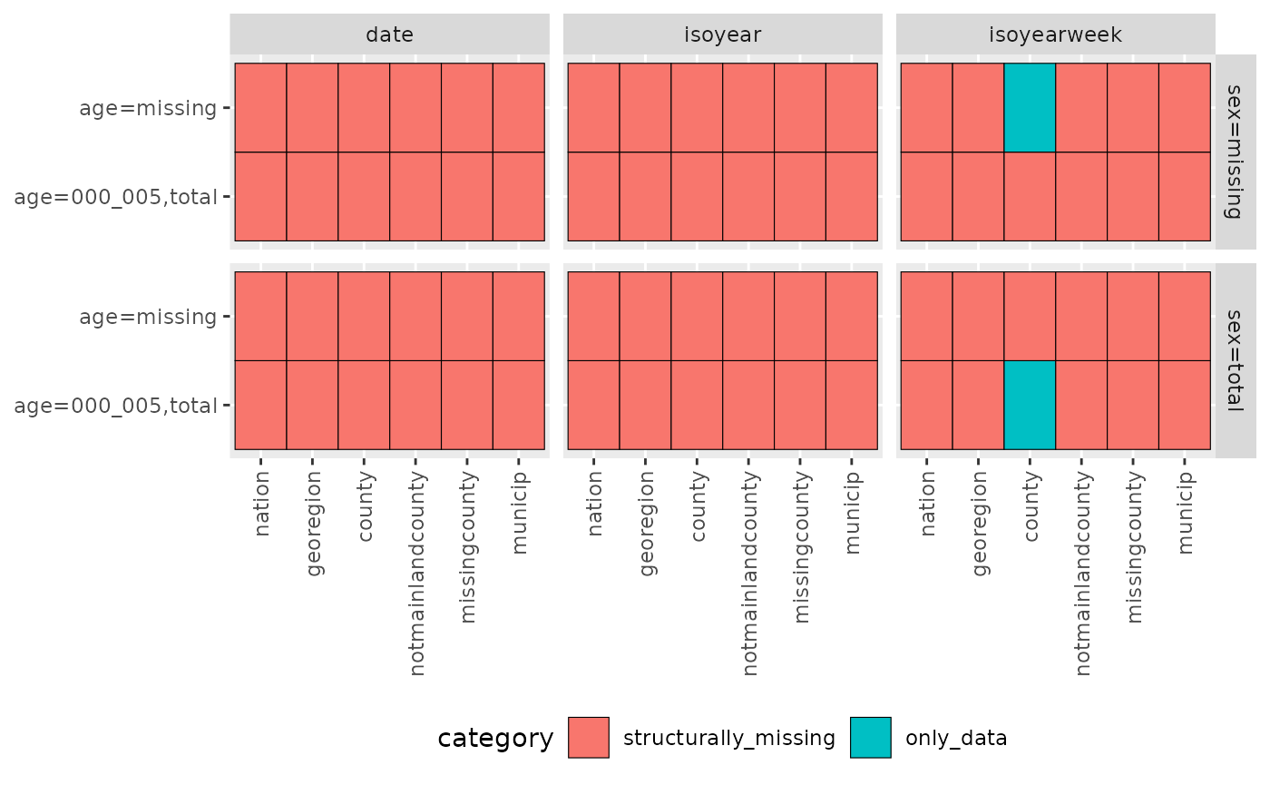
Identifying the data structure of one column
cstidy::identify_data_structure() inspects a single
column and returns a plottable object.
cstidy::generate_test_data() |>
  cstidy::set_csfmt_rts_data_v2() |>
  cstidy::identify_data_structure("deaths_n") |>
  plot()