The pipeline: from incomplete counts to published numbers

Surveillance counts arrive late. A case that belongs to week W may only be reported in week W, W+1, W+2, and so on. So the newest weeks always look lower than they will turn out to be. Anything you measure on them — a trend, an intensity level, an alert — inherits that dip.

This vignette runs one series through the whole of csalert. It fills in the weeks that are still arriving, checks how far that filling can be trusted, and ends with numbers you could publish.

Three shapes carry the run.

csfmt_reporting_triangle_v3 — the input. One cell per reference week and reporting week, so it records what was reported when.
csfmt_ensemble_v3 — the working format. It holds $data, plus one matrix of Monte-Carlo $draws per measure (rows = weeks, columns = simulations). Each stage adds columns to the draws, so the uncertainty is carried forward rather than recomputed.
a quantile collapse of those draws — the output, optionally healed into cstidy::csfmt_rts_data_v3 for the usual plots and tables.

One rule: every stage takes the ensemble and returns it

That rule explains the shape of everything below.

Every analytical stage takes a csfmt_ensemble_v3 and returns a csfmt_ensemble_v3. ens_collapse() is terminal: it reduces the draws to quantiles, and a collapsed table is output, never input.

So the canonical pipeline is a single chain through the ensemble:

csfmt_reporting_triangle_v3
  -> nowcast_quasipoisson_v1  OR  nowcast_passthrough_to_ensemble_v1
  -> [ens_add_rate]              # when a denominator exists
  -> [short_term_trend]          # growth rate + P(increasing)
  -> [mem_thresholds_v1]         # MEM intensity
  -> [signal_detection_hlm]      # per-draw exceedance
  -> ens_collapse(heal = TRUE)   # ensemble -> quantiles -> csfmt_rts_data_v3

The bracketed stages are optional and order-flexible among themselves; each one adds draw columns and hands the ensemble on. What you cannot do is collapse and then carry on. A collapsed table holds quantiles, not draws. Feed it back into short_term_trend() and you cannot recover a per-draw trend or a P(increasing). That is by design, not a gap — the draws are the uncertainty, and the collapse is where you spend them.

The series below is synthetic, and it runs the whole chain:

Nowcast — fill in the recent weeks that are still being reported.
Validation — replay the method against what was known in the past.
Reporting completion — read the reporting delay off the triangle itself.
Rate — a nowcasted numerator over a nowcasted denominator, per draw.
Short-term trend — the recent slope of that rate, per draw.
MEM intensity — seasonal intensity thresholds, classified per draw.
Signal detection — historical-limits exceedance, per draw.
Collapse — quantiles, healed into cstidy::csfmt_rts_data_v3.

Stages 4 to 8 are the ensemble chain above. Stages 2 and 3 are not. They take the triangle, not the ensemble, because they ask about the reporting process rather than about the completed counts. Keep that split in mind. Anything that asks how the data arrives reads the triangle; anything that asks what the data says reads the ensemble.

When you set up a new indicator, run stage 3 first: it is what supports the choice of max_delay that everything else then uses.

library(data.table)
#> 
#> Attaching package: 'data.table'
#> The following object is masked from 'package:base':
#> 
#>     %notin%
library(csalert)
#> csalert 2026.8.7
#> https://niphr.github.io/csalert/

A synthetic reporting triangle

Real surveillance data arrives with a delay: a case with reference week W may only be reported in week W, W+1, W+2, and so on. The generator below simulates a laboratory indicator from ISO week 2019-35 to 2024-18. That span is five winter seasons, which is what stages 6 and 7 need. It has a reporting speed-up built in at the start of ISO year 2024. Stage 3 recovers that change from the triangle alone.

It emits a numerator and a denominator: tests taken, and how many were positive. Simulating positives as a binomial conditional on the tests keeps the numerator a subset of the denominator, which is what makes their ratio a proportion. Two independent Poissons would not be. Each test carries one reporting delay, so a result and its test land in the same triangle cell.

set.seed() is called inside the generator, not beside it. A seed set outside a function that is called more than once leaves the second call running on a different stream. The resulting Monte-Carlo noise reads as signal.

sim_reports <- function(first_ref = "2019-35",
                        last_ref = "2024-18",
                        delay_slow = c(0.45, 0.30, 0.15, 0.07, 0.03),
                        delay_fast = c(0.70, 0.20, 0.06, 0.03, 0.01),
                        seed = 1L) {
  set.seed(seed)                                    # pinned inside, see above
  weeks <- cstime::dates_by_isoyearweek$isoyearweek
  i0 <- match(first_ref, weeks)
  i1 <- match(last_ref, weeks)
  rows <- lapply(i0:i1, function(ri) {
    ref <- weeks[ri]
    s <- cos(2 * pi * (cstime::isoyearweek_to_isoweek_n(ref) - 5) / 52)  # winter peak
    n_tests <- rpois(1, 400 + 120 * s)
    positive <- rbinom(n_tests, 1, stats::plogis(-2.2 + 1.1 * s))        # subset of tests
    p <- if (cstime::isoyearweek_to_isoyear_n(ref) <= 2023) delay_slow else delay_fast
    data.table(
      isoyearweek_reference = ref,
      isoyearweek_reporting = weeks[ri + sample(0:4, n_tests, TRUE, p)],
      positive = positive
    )
  })
  # "today" is the last reference week: drop what has not been reported yet, so
  # the most recent weeks are still incomplete -- the problem a nowcast solves
  rbindlist(rows)[isoyearweek_reporting <= weeks[i1]]
}

reports <- sim_reports()
triangle_long <- reports[, .(numerator = sum(positive), denominator = .N),
                         by = .(isoyearweek_reference, isoyearweek_reporting)]
triangle_long[, `:=`(indicator_tag = "lab_flu", location_code = "nation",
                     age = "total", sex = "total")]
head(triangle_long, 4)
#>    isoyearweek_reference isoyearweek_reporting numerator denominator
#>                   <char>                <char>     <int>       <int>
#> 1:               2019-35               2019-35         1         132
#> 2:               2019-35               2019-39         0          12
#> 3:               2019-35               2019-36         3          78
#> 4:               2019-35               2019-38         0          24
#>    indicator_tag location_code    age    sex
#>           <char>        <char> <char> <char>
#> 1:       lab_flu        nation  total  total
#> 2:       lab_flu        nation  total  total
#> 3:       lab_flu        nation  total  total
#> 4:       lab_flu        nation  total  total
c(cells = nrow(triangle_long),
  numerator_never_exceeds_denominator =
    all(triangle_long$numerator <= triangle_long$denominator))
#>                               cells numerator_never_exceeds_denominator 
#>                                1215                                   1

Wrap it as a csfmt_reporting_triangle_v3. The as-of boundary is read from the data — it is the newest reporting week present, not the system clock.

tri <- csfmt_reporting_triangle_v3(
  triangle_long,
  id_cols       = c("indicator_tag", "location_code", "age", "sex"),
  reference_col = "isoyearweek_reference",
  reporting_col = "isoyearweek_reporting",
  value_col     = "numerator"
)
c(as_of = attr(tri, "as_of"),
  newest_reporting_week = max(triangle_long$isoyearweek_reporting))
#>                 as_of newest_reporting_week 
#>             "2024-18"             "2024-18"

max_delay is the delay horizon used by stages 1 to 3 below. Stage 3 shows how to choose it from the data; 5 weeks is the right answer for this series.

max_delay <- 5L

1. Nowcast

Estimand. For each reference week, the total that will have been reported at delays 0 .. max_delay - 1 — that is, by the end of ISO week reference_week + max_delay - 1. This is a horizon-capped total, not the eventual total. Anything reported later than max_delay - 1 weeks is outside the estimand, and no amount of nowcasting recovers it. Stage 3 is how you check that the horizon is wide enough for the difference to be small. For a settled week the quantity is already observed. For the most recent weeks it is not, and the nowcast is a predictive distribution over it.

nowcast_quasipoisson_v1() is a discriminative (regression) engine. For each number of weeks a reference week has been observed, it fits one regression on the settled weeks. That regression is quasipoisson with an identity link, of the settled total on the counts reported so far:

total ~ n[delay 0] + n[delay 1] + ... + n[delay h]

R’s default intercept is present in that formula and is fitted. There is no per-week magnitude parameter, so the recent weeks do not each carry their own noisy level. Draws combine the fit’s parameter uncertainty with a dispersion-matched negative binomial. delay_window (default 26 weeks) restricts training to the settled weeks within roughly that span. The partial-to-total mapping can then follow a reporting regime that changes — as this series’ does.

denominator_col nowcasts a second measure alongside the numerator, on the same draw axis. Stage 4 needs it: a rate is only coherent if both its parts are completed in the same Monte-Carlo world.

set.seed(2)
ens <- nowcast_quasipoisson_v1(tri, max_delay = max_delay, n_sim = 500,
                               denominator_col = "denominator")
ens
#> <csfmt_ensemble_v3> 245 rows | 1 series | draws: numerator_nowcasted, denominator_nowcasted

Collapse the draws to a quantile summary. original is the count reported so far; the settled weeks sit exactly on it, the recent weeks are completed above it.

q <- ens_collapse(ens, probs = c(0.05, 0.5, 0.95))
tail(q[, .(isoyearweek, original,
           lo  = numerator_nowcasted_q05x0,
           med = numerator_nowcasted_q50x0,
           hi  = numerator_nowcasted_q95x0)], 8)
#>    isoyearweek original    lo   med    hi
#>         <char>    <num> <num> <num> <num>
#> 1:     2024-11      100   100   100   100
#> 2:     2024-12       94    94    94    94
#> 3:     2024-13       69    69    69    69
#> 4:     2024-14       67    67    67    67
#> 5:     2024-15       50    50    50    61
#> 6:     2024-16       47    47    49    62
#> 7:     2024-17       43    43    46    57
#> 8:     2024-18       23    29    46    66

The settled weeks are pinned to their observed total, so they have no band at all. Only the incomplete weeks at the right-hand edge carry one:

show <- tail(q, 30)
xs   <- seq_len(nrow(show))
plot(xs, show$numerator_nowcasted_q50x0, type = "n",
     ylim = range(show$numerator_nowcasted_q05x0, show$numerator_nowcasted_q95x0),
     xlab = "week (last 30)", ylab = "weekly total (nowcast)")
polygon(c(xs, rev(xs)),
        c(show$numerator_nowcasted_q05x0, rev(show$numerator_nowcasted_q95x0)),
        col = grDevices::adjustcolor("steelblue", 0.25), border = NA)
lines(xs, show$numerator_nowcasted_q50x0, lwd = 2, col = "steelblue4")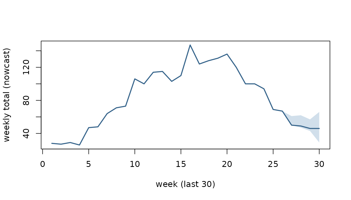

Keep the reference weeks: the later stages index off them.

weeks     <- cstime::dates_by_isoyearweek$isoyearweek
ref_weeks <- q$isoyearweek

2. Validation: replay the method against the past

This stage and the next take the triangle, not the ensemble. They ask how the data arrives. That is a property of the reporting process, and it is destroyed the moment the delay axis is collapsed into weekly totals.

The triangle records when every count arrived. So you can reconstruct what was known at any past week and replay the engine against it, without a second dated extract.

That reconstruction is exact only for an append-only reporting system: one where a count, once filed, keeps its original reporting week forever. Real systems also issue retrospective corrections, delete records and reclassify cases. None of those leave a trace in the current triangle. A case reclassified last month looks as though it was always classified that way. Where such revisions matter, replay understates how much the published numbers actually moved. A dated archive of extracts is the only way to measure it.

nowcast_censor() does the rewind. It returns a csfmt_reporting_triangle_v3 with every cell reported after the given week dropped, and its as-of boundary moved back:

past <- nowcast_censor(tri, as_of = ref_weeks[length(ref_weeks) - 8L])
c(now  = attr(tri, "as_of"),  then      = attr(past, "as_of"),
  rows_now = nrow(tri),       rows_then = nrow(past))
#>       now      then  rows_now rows_then 
#> "2024-18" "2024-10"    "1215"    "1175"

nowcast_truth() supplies the target. It returns a two-column data.table (reference, truth) of each reference week’s total summed over delays 0 .. max_delay - 1, keeping only the weeks old enough for that total to be settled. The newest weeks are absent by design: they have no truth to be scored against yet.

truth <- nowcast_truth(tri, max_delay = max_delay)
tail(truth, 3)
#>    reference truth
#>       <char> <num>
#> 1:   2024-12    94
#> 2:   2024-13    69
#> 3:   2024-14    67
c(reference_weeks = length(ref_weeks), settled = nrow(truth))
#> reference_weeks         settled 
#>             245             241

A method is any function f(triangle) -> csfmt_ensemble_v3 with its own parameters baked in. That one-argument contract is what lets engines with different signatures be replayed and compared through the same harness.

method_qp <- function(x) nowcast_quasipoisson_v1(x, max_delay = max_delay, n_sim = 500)
as_of_weeks <- tail(ref_weeks, 30)

nowcast_backtest() runs the replay and returns the raw scored quantiles: one long row per reference x as_of x horizon x quantile_level, with the predicted value. horizon is weeks between the reference week and the as-of week, so horizon 0 is the current, least-observed week.

bt <- nowcast_backtest(
  tri, method_qp,
  max_delay   = max_delay,
  as_of_weeks = as_of_weeks,
  horizons    = 0:3,
  probs       = c(0.05, 0.25, 0.5, 0.75, 0.95),
  seed        = 1
)
head(bt, 4)
#>    reference   as_of horizon quantile_level predicted
#>       <char>  <char>   <int>          <num>     <num>
#> 1:   2023-38 2023-41       3           0.05     24.00
#> 2:   2023-39 2023-41       2           0.05     19.00
#> 3:   2023-40 2023-41       1           0.05     14.00
#> 4:   2023-41 2023-41       0           0.05     22.95
nrow(bt)
#> [1] 600

nowcast_evaluate_v1() wraps that replay and scores it, joining each forecast to its settled truth. It returns one row per group (default: per horizon) per method:

n — the number of scored forecasts behind that row.
coverage_50, coverage_90 — the measured share of settled truths that fell inside the nominal 50% and 90% central intervals on this replay. These are sample quantities, not a property of the construction.
median_signed, median_abs, q05, q95, p_gt_25, p_gt_50 — the revision of the published median relative to the settled truth, as a fraction of the truth. median_signed is the median signed relative revision across the replayed forecasts, not a mean, so it is not the bias in the usual expected-error sense. p_gt_25 and p_gt_50 are empirical exceedance proportions: the share of replayed forecasts whose absolute relative revision exceeded 0.25 and 0.50. They are not probabilities of anything.

Passing a named list of methods replays every method over the same reference and as-of weeks, so the comparison is paired by forecast unit. seed makes each method’s own run reproducible. It does not by itself create common random numbers across methods; that would need the algorithms to consume compatible variates. Here it cannot: nowcast_passthrough_to_ensemble_v1() draws no random numbers at all. Racing against it — it does no completion and just republishes the counts reported so far — makes the numbers readable:

ev <- nowcast_evaluate_v1(
  tri,
  methods = list(
    quasipoisson = method_qp,
    passthrough  = function(x) nowcast_passthrough_to_ensemble_v1(x, max_delay = max_delay)
  ),
  max_delay   = max_delay,
  as_of_weeks = as_of_weeks,
  horizons    = 0:3,
  seed        = 1
)
ev[, .(method, horizon, n, coverage_50, coverage_90, median_signed, median_abs)]
#>          method horizon     n coverage_50 coverage_90 median_signed median_abs
#>          <char>   <int> <int>       <num>       <num>         <num>      <num>
#> 1: quasipoisson       3    29       1.000       1.000        0.0000     0.0161
#> 2: quasipoisson       2    28       0.893       1.000        0.0039     0.0371
#> 3: quasipoisson       1    27       0.630       0.963        0.0448     0.0660
#> 4: quasipoisson       0    26       0.346       0.692        0.1421     0.1937
#> 5:  passthrough       3    29       0.310       0.310       -0.0100     0.0100
#> 6:  passthrough       2    28       0.036       0.036       -0.0594     0.0594
#> 7:  passthrough       1    27       0.000       0.000       -0.1544     0.1544
#> 8:  passthrough       0    26       0.000       0.000       -0.3842     0.3842

Read that table as a measurement on this sample and no further. Each row rests on 26 to 29 scored weeks of one synthetic series. That is far too few to characterise either engine. A coverage estimate from 26 scored weeks has a standard error of roughly 0.06 at 0.9 and 0.10 at 0.5. That is before any dependence between overlapping windows is allowed for.

What the comparison does show is the shape of the problem. What construction guarantees for the passthrough is only this: each of its forecasts is no greater than the settled truth. A count that is still arriving cannot exceed its own total. Every individual revision is therefore zero or negative.

That alone does not force a strictly negative median at a given horizon. If more than half the weeks were already complete, the median would be exactly zero. It also does not order the horizons. The negative median_signed at all four horizons, and horizon 0 being the worst, are findings on this sample, not consequences of the construction.

Its coverage_50 and coverage_90 are equal because a single draw gives it no interval at all. The “interval” is a point. It covers the truth only when the republished count already equals it. At horizon 3 that happens on the weeks where nothing arrived at delay 4.

The engine’s horizon-0 row is worth stopping on

The quasipoisson engine’s horizon-0 coverage is well below nominal, and its median_signed is positive — it is over-completing. That is not a random dip. The replay window above ends at the as-of week, so it straddles the reporting speed-up this series has at the start of ISO 2024. The engine trains on the 26 preceding settled weeks. Learn the completion factors of a slow regime, then apply them to partial counts from a fast one. You scale up counts that were already nearly complete.

The contrast is visible if the replay is restricted to as-of weeks that sit entirely inside the slow regime:

slow_weeks <- tail(ref_weeks[cstime::isoyearweek_to_isoyear_n(ref_weeks) == 2023], 30)
c(from = slow_weeks[1], to = slow_weeks[length(slow_weeks)])
#>      from        to 
#> "2023-23" "2023-52"
nowcast_evaluate_v1(tri, method_qp, max_delay = max_delay,
                    as_of_weeks = slow_weeks, horizons = 0:3, seed = 1)[
  , .(horizon, n, coverage_50, coverage_90, median_signed, median_abs)]
#>    horizon     n coverage_50 coverage_90 median_signed median_abs
#>      <int> <int>       <num>       <num>         <num>      <num>
#> 1:       3    30       1.000       1.000        0.0000     0.0000
#> 2:       2    30       0.933       1.000        0.0000     0.0596
#> 3:       1    30       0.833       1.000        0.0665     0.0909
#> 4:       0    30       0.533       0.867        0.1056     0.1909

Horizon 0 recovers, and the bias changes sign. Read that as a demonstration of the mechanism, not as a measured effect size. The two windows also differ in which weeks and which part of the season they cover. A sample of 26 to 30 scored weeks cannot separate those from the regime change. The general lesson is the one delay_window exists for: a nowcast engine is only as current as the reporting behaviour it was trained on. Stage 3 is how you find out when that behaviour moved.

nowcast_estimate_calibration_v1() reports the same per-horizon coverage alongside an interval-scaling factor learned from the replay. Its documentation is explicit that this is an empirical rescaling and not split conformal, so the factor carries no finite-sample coverage guarantee.

3. Reporting completion: how fast does the data actually arrive?

What `pct_delayD` counts

pct_delay0 is the share of a reference week’s cases that were reported during that same ISO week. Delay 0 is the reference week itself, not the week after it. In general:

pct_delayD is the pooled share of a reference week’s cases reported by the end of ISO week reference_week + D.

The columns are indexed by delay, 0-based, so the index in the name is the delay it reports. There are max_delay of them and the highest is pct_delay<max_delay - 1>, matching the triangle’s own delay axis. Each is the delay ECDF read at one delay, with no interpolation. mean_delay is on the same axis and in whole weeks, so a week whose cases all arrive at delay 0 has mean_delay 0, not 1.

A triangle with a known answer settles it. Below, each reference week generates exactly 50 at delay 0, 30 at delay 1 and 20 at delay 2. The result is right-truncated at the newest reporting week, the way real data is:

i <- match("2023-01", weeks)
pin <- data.table(
  isoyearweek_reference = weeks[i + rep(0:29, each = 3)],
  isoyearweek_reporting = weeks[i + rep(0:29, each = 3) + rep(0:2, 30)],
  numerator = rep(c(50, 30, 20), 30),
  indicator = "pinned", location = "nation", age = "total", sex = "total"
)
pin <- pin[isoyearweek_reporting <= weeks[i + 29]]
tri_pin <- csfmt_reporting_triangle_v3(
  pin, id_cols = c("indicator", "location", "age", "sex")
)
reporting_completion_v1(tri_pin, max_delay = 3)[
  , .(n_settled, mean_delay, complete_by_md, pct_delay0, pct_delay1, pct_delay2)]
#>    n_settled mean_delay complete_by_md pct_delay0 pct_delay1 pct_delay2
#>        <int>      <num>          <num>      <num>      <num>      <num>
#> 1:        28        0.7              1         50         80        100

pct_delay0 is 50, not 80: it is the delay-0 share, the reports that arrived in the reference week itself. pct_delay1 is 80 — cumulative through delay 1. mean_delay is 0*0.50 + 1*0.30 + 2*0.20 = 0.70.

Coming from an older script? These columns used to be named pct_w1, pct_w2, …, which counted weeks-observed from 1. So no number in a column name ever equalled the delay it stood for. Your pct_w1 is now pct_delay0, pct_w2 is pct_delay1, and so on. The old names are gone rather than redefined, so old code errors on a missing column instead of quietly returning a different week.

n_settled is 28, not 30. Age eligibility is the first filter. A reference week is eligible once as_of_week - reference_week >= max_delay - 1, which excludes the two most recent of those 30. A second filter then drops any eligible week whose total within the horizon is zero, and n_settled counts what survives both. Here no week is empty, so the age rule alone accounts for the number — and the same holds on the working triangle:

age <- match(attr(tri, "as_of"), weeks) - match(ref_weeks, weeks)
completion <- reporting_completion_v1(tri, max_delay = max_delay)
c(age_eligible = sum(age >= max_delay - 1L), reported = completion$n_settled)
#> age_eligible     reported 
#>          241          241

They agree only because this series has no zero-count weeks. On an indicator with quiet weeks — a rare pathogen, a small stratum — n_settled will be the smaller of the two. A period slice with fewer than three surviving weeks is dropped from the output entirely.

A worked reference week

Take reference week 2023-07. cstime gives its calendar dates, and the two weeks after it:

cstime::dates_by_isoyearweek[
  isoyearweek %in% c("2023-07", "2023-08", "2023-09"),
  .(isoyearweek, isoyear, mon, thu, sun)
]
#>    isoyearweek isoyear        mon        thu        sun
#>         <char>   <int>     <Date>     <Date>     <Date>
#> 1:     2023-07    2023 2023-02-13 2023-02-16 2023-02-19
#> 2:     2023-08    2023 2023-02-20 2023-02-23 2023-02-26
#> 3:     2023-09    2023 2023-02-27 2023-03-02 2023-03-05

For a case whose reference week is 2023-07:

statistic	covers reports up to	which is
`pct_delay0`	end of ISO week 2023-07	Sunday 2023-02-19
`pct_delay1`	end of ISO week 2023-08	Sunday 2023-02-26
`pct_delay2`	end of ISO week 2023-09	Sunday 2023-03-05

So pct_delay0 is a statement about the seven days from Monday 2023-02-13. pct_delay1 is about the 14 days from that same Monday, not the seven days of week 2023-08 on their own. The columns are cumulative.

Which day of the week you run it on

The day of the week does not change the delay arithmetic at all. Delay is computed from the two ISO-week labels only. So every day of a week carries the same label and lands in the same delay bucket:

days <- seq(as.Date("2023-02-13"), as.Date("2023-02-19"), by = "day")
data.table(date = days, weekday = weekdays(days),
           isoyearweek = cstime::date_to_isoyearweek_c(days))
#>          date   weekday isoyearweek
#>        <Date>    <char>      <char>
#> 1: 2023-02-13    Monday     2023-07
#> 2: 2023-02-14   Tuesday     2023-07
#> 3: 2023-02-15 Wednesday     2023-07
#> 4: 2023-02-16  Thursday     2023-07
#> 5: 2023-02-17    Friday     2023-07
#> 6: 2023-02-18  Saturday     2023-07
#> 7: 2023-02-19    Sunday     2023-07

Both runs put a report filed that week at delay 0 for reference week 2023-07, at delay 1 for 2023-06, and so on. Nothing in the pipeline reads the system clock: the as-of boundary comes from the newest reporting week present in the data.

The phrase present in the data carries a condition worth stating. as_of is max(reporting_week). A Monday run and a Friday run therefore agree on as_of = "2023-07" under one condition. The Monday extract must already contain at least one report filed in week 2023-07.

If it contains none — a plausible Monday morning on a slow indicator — as_of silently falls back to "2023-06". Every week’s age shifts by one, and one more reference week is treated as settled. That is a different analysis, not a smaller one, and nothing in the output announces it.

What the day does change is how much of the current week’s reporting has landed. On Monday almost none of it has landed. In this illustration all of it is in by Sunday. That assumes the extract is taken after the week closes, and that the system files everything within the week it belongs to. Neither is guaranteed in general.

In a Monday extract every cell whose reporting week is the current week is still filling. That is the delay-0 cell of the current reference week most visibly. The same holds for the delay-1 cell of last week, the delay-2 cell of the week before, and so on.

That matters for the completion table in one narrow place, and it is worth being precise about which. Thin the current week’s reports down to 15%, as a Monday extract would see them, and rebuild:

set.seed(5)
monday <- reports[isoyearweek_reporting != attr(tri, "as_of") | runif(.N) < 0.15]
tl_mon <- monday[, .(numerator = sum(positive), denominator = .N),
                 by = .(isoyearweek_reference, isoyearweek_reporting)]
tl_mon[, `:=`(indicator_tag = "lab_flu", location_code = "nation",
              age = "total", sex = "total")]
tri_mon <- csfmt_reporting_triangle_v3(
  tl_mon, id_cols = c("indicator_tag", "location_code", "age", "sex")
)

rbind(
  cbind(extract = "Sunday (week complete)",
        reporting_completion_v1(tri, max_delay = max_delay)[
          , .(n_settled, mean_delay, pct_delay0, pct_delay1, pct_delay2, pct_delay3)]),
  cbind(extract = "Monday (15% of the week in)",
        reporting_completion_v1(tri_mon, max_delay = max_delay)[
          , .(n_settled, mean_delay, pct_delay0, pct_delay1, pct_delay2, pct_delay3)])
)
#>                        extract n_settled mean_delay pct_delay0 pct_delay1
#>                         <char>     <int>      <num>      <num>      <num>
#> 1:      Sunday (week complete)       241       0.88       47.3       76.7
#> 2: Monday (15% of the week in)       241       0.88       47.3       76.7
#>    pct_delay2 pct_delay3
#>         <num>      <num>
#> 1:       90.6       97.1
#> 2:       90.6       97.1

The pooled curve barely moves, and n_settled is identical, because the current reference week is never in the settled set. For any max_delay of 2 or more its age is 0, which is below the max_delay - 1 threshold. So it contributes nothing to pct_delayD whichever day you run on. (A max_delay of 1 leaves a single delay bucket, no completion to measure, and no useful summary; use 2 or more).

At most one reference week can have its settled total affected: the newest settled one. Its last delay cell — delay max_delay - 1 — is still being reported during the current week. Every older week finished reporting earlier; every newer week is not settled. Count the weeks that actually moved, rather than assuming it is one:

cmp <- merge(nowcast_truth(tri, max_delay), nowcast_truth(tri_mon, max_delay),
             by = "reference", suffixes = c("_sunday", "_monday"))
cmp[(.N - 2):.N]
#> Key: <reference>
#>    reference truth_sunday truth_monday
#>       <char>        <num>        <num>
#> 1:   2024-12           94           94
#> 2:   2024-13           69           69
#> 3:   2024-14           67           67
cmp[truth_sunday != truth_monday]
#> Key: <reference>
#> Empty data.table (0 rows and 3 cols): reference,truth_sunday,truth_monday

On this series, none did — and the reason is worth seeing, because it bounds the whole effect. The only cell at risk is the delay-4 numerator of the newest settled week. In the fast 2024 regime, delay 4 carries 1% of a week’s tests:

newest_settled <- weeks[match(attr(tri, "as_of"), weeks) - (max_delay - 1L)]
triangle_long[isoyearweek_reference == newest_settled &
              isoyearweek_reporting == attr(tri, "as_of"),
              .(isoyearweek_reference, isoyearweek_reporting, numerator, denominator)]
#>    isoyearweek_reference isoyearweek_reporting numerator denominator
#>                   <char>                <char>     <int>       <int>
#> 1:               2024-14               2024-18         0           3

Five tests, none of them positive. Thinning zero positives leaves zero, so the numerator’s settled total cannot move. The weekday effect is bounded by the mass sitting in the last delay bucket. Widen max_delay past where reporting actually finishes and that bucket empties. That is why the effect vanishes here, and why it did not vanish on a series with a heavier tail.

None of this generalises, and the two reasons it vanishes here are both about scale. The at-risk cell is one week’s last delay bucket, diluted into a pool of 241 settled weeks. That bucket is also nearly empty, because max_delay is wide enough. Shrink the series, shrink the horizon, or give the indicator a heavier reporting tail, and the same mechanism becomes material. A period slice with the minimum three qualifying weeks gives that one cell a third of the weight.

The general statement is the conditional one. A mid-week extract undercounts the newest settled week’s total by whatever share of its last delay bucket has not arrived. That total is what nowcast_truth() scores a backtest against. So run the backtest off an end-of-week extract. The alternative is to measure the gap on your own series, rather than assuming it is as small as it is here.

“As of today”, for the weeks on screen

With as_of = 2024-18 and max_delay = 5, the reference weeks split three ways:

data.table(
  isoyearweek = ref_weeks,
  weeks_observed = age + 1L,
  status = fifelse(age >= max_delay - 1L, "settled",
           fifelse(age > 0L, "still filling", "current week"))
)[, .N, keyby = status]
#> Key: <status>
#>           status     N
#>           <char> <int>
#> 1:  current week     1
#> 2:       settled   241
#> 3: still filling     3

Four weeks are not settled: three still filling, plus the current week, which has only its delay-0 reports. Those are the weeks the nowcast in stage 1 completed, and the weeks the completion table declines to learn from. The completed weeks are the ones whose nowcast rises above the count reported so far:

q[numerator_nowcasted_q95x0 > original, isoyearweek]
#> [1] "2024-15" "2024-16" "2024-17" "2024-18"

Reporting drift: `period = "year"`

period = "year" returns one row per qualifying ISO year, and it is how you see a reporting system speeding up or slowing down. One pooled curve cannot: it averages the regimes together and describes neither.

“Qualifying” is load-bearing. A period slice needs at least three settled weeks with a non-zero within-horizon total. A slice below that is dropped from the result, with no warning and no placeholder row. A year at the edge of the series — the one your data starts or ends in — is the usual casualty. A missing year means too few weeks, never zero delay.

reporting_completion_v1(tri, max_delay = max_delay, period = "year")[
  , .(period, n_settled, mean_delay, pct_delay0, pct_delay1, pct_delay2, pct_delay3)]
#>    period n_settled mean_delay pct_delay0 pct_delay1 pct_delay2 pct_delay3
#>    <char>     <int>      <num>      <num>      <num>      <num>      <num>
#> 1:   2019        18       0.96       44.4       73.5       89.4       96.4
#> 2:   2020        53       0.95       44.2       75.0       89.8       96.3
#> 3:   2021        52       0.92       45.5       75.6       89.8       97.0
#> 4:   2022        52       0.90       45.1       76.0       91.4       97.2
#> 5:   2023        52       0.95       44.4       74.5       89.0       97.0
#> 6:   2024        14       0.49       67.7       89.1       95.7       98.8

That is the change built into sim_reports(), recovered from the triangle. Five consecutive ISO years sit within a couple of points of each other — pct_delay0 around 43 to 45, mean_delay around 0.95. Then 2024 steps to about 69% and 0.45. A flat run followed by a step is what a genuine regime change looks like. A single year out of line with its neighbours is usually noise.

The pooled row from the previous table reports pct_delay0 of 47.3. That is close to the five slow years only because they outnumber the fast one five to one. It is not a compromise between the regimes. It is the old regime with a little contamination, and it will drift year by year as 2024 accumulates weeks.

The stratification is by ISO year, not calendar year, and the ISO year of a week is the calendar year of its Thursday. That decides which year owns a boundary week:

cstime::dates_by_isoyearweek[
  isoyearweek %in% c("2022-52", "2023-01"), .(isoyearweek, isoyear, mon, thu, sun)
]
#>    isoyearweek isoyear        mon        thu        sun
#>         <char>   <int>     <Date>     <Date>     <Date>
#> 1:     2022-52    2022 2022-12-26 2022-12-29 2023-01-01
#> 2:     2023-01    2023 2023-01-02 2023-01-05 2023-01-08

ISO week 2022-52 has its Thursday on 2022-12-29, so it belongs to ISO year 2022 even though its Sunday, 2023-01-01, is a calendar-2023 date. ISO week 2023-01 has its Thursday on 2023-01-05 and belongs to 2023.

period = "month" slices finer and localises when a change happened. It uses the same Thursday rule to decide which calendar month owns a week that straddles two:

tail(reporting_completion_v1(tri, max_delay = max_delay, period = "month")[
  , .(period, n_settled, mean_delay, pct_delay0, pct_delay1)], 6)
#>     period n_settled mean_delay pct_delay0 pct_delay1
#>     <char>     <int>      <num>      <num>      <num>
#> 1: 2023-10         4       0.83       51.0       76.0
#> 2: 2023-11         5       0.88       46.5       79.7
#> 3: 2023-12         4       1.02       43.8       71.2
#> 4: 2024-01         4       0.52       66.3       89.1
#> 5: 2024-02         5       0.48       67.4       89.0
#> 6: 2024-03         4       0.50       68.0       88.2

The step lands between 2023-12 and 2024-01. Note the small n_settled per month — four or five weeks — so a single month’s row is noisy; read the sequence, not one row.

Every number here is conditional on `max_delay`

This is the trap, and it is structural rather than a tuning subtlety. reporting_completion_v1() works from a triangle that has already had every cell with delay >= max_delay discarded. So the denominator is the total that arrived within the horizon, not the eventual total. Two consequences follow, and they hold whatever the real reporting tail looks like:

complete_by_md is the last cumulative fraction of that same truncated total, so it is 1.
the last column, pct_delay<max_delay - 1>, is that fraction as a percentage, so it is 100.

Neither can detect reporting that dribbles in past the horizon. Rather than assert that, check it — here across max_delay 2 through 8 on this triangle, reading the last column by name each time:

sens <- rbindlist(lapply(2:8, function(md) {
  r <- reporting_completion_v1(tri, max_delay = md)
  data.table(max_delay = md, n_settled = r$n_settled, mean_delay = r$mean_delay,
             complete_by_md = r$complete_by_md,
             last_col = paste0("pct_delay", md - 1L),
             last_pct = r[[paste0("pct_delay", md - 1L)]],
             pct_delay0 = r$pct_delay0, pct_delay1 = r$pct_delay1,
             pct_delay2 = r$pct_delay2)
}), fill = TRUE)
sens
#>    max_delay n_settled mean_delay complete_by_md   last_col last_pct pct_delay0
#>        <int>     <int>      <num>          <num>     <char>    <num>      <num>
#> 1:         2       244       0.38              1 pct_delay1      100       62.0
#> 2:         3       243       0.63              1 pct_delay2      100       52.4
#> 3:         4       242       0.79              1 pct_delay3      100       48.9
#> 4:         5       241       0.88              1 pct_delay4      100       47.3
#> 5:         6       240       0.89              1 pct_delay5      100       47.2
#> 6:         7       239       0.89              1 pct_delay6      100       47.1
#> 7:         8       238       0.89              1 pct_delay7      100       46.9
#>    pct_delay1 pct_delay2
#>         <num>      <num>
#> 1:      100.0         NA
#> 2:       84.7      100.0
#> 3:       79.0       93.3
#> 4:       76.7       90.6
#> 5:       76.6       90.6
#> 6:       76.6       90.5
#> 7:       76.4       90.5
c(complete_by_md_always_1 = all(sens$complete_by_md == 1),
  last_pct_always_100     = all(sens$last_pct == 100))
#> complete_by_md_always_1     last_pct_always_100 
#>                    TRUE                    TRUE

The same holds inside every period slice, which is where it is easiest to mistake for a finding:

per <- rbindlist(lapply(c("all", "year", "month"), function(p) {
  r <- reporting_completion_v1(tri, max_delay = max_delay, period = p)
  data.table(period_arg = p, rows = nrow(r),
             complete_by_md_all_1 = all(r$complete_by_md == 1),
             pct_delay4_all_100 = all(r$pct_delay4 == 100))
}))
per
#>    period_arg  rows complete_by_md_all_1 pct_delay4_all_100
#>        <char> <int>               <lgcl>             <lgcl>
#> 1:        all     1                 TRUE               TRUE
#> 2:       year     6                 TRUE               TRUE
#> 3:      month    55                 TRUE               TRUE

The diagnostic that does work is the max_delay sweep itself. Read the sens table above down its rows. mean_delay rises from 0.38 at max_delay 2 to 0.88 at 5, then moves only to 0.89 at 8. pct_delay0 falls from 61.8 to 47.3 and then drifts to 46.8. That flattening is what supports max_delay <- 5L here — it is a sensitivity analysis, not a proof.

A mean_delay that kept climbing would be clear evidence the tail was still being cut off. A plateau is weaker evidence in the other direction, because a genuinely sparse tail and a shifting settled-week composition both flatten the curve too.

Two cautions on reading that sweep:

The short horizons are not merely imprecise, they are biased optimistic. pct_delay0 at max_delay 2 reads 61.8% because it conditions on the cases that arrived within two weeks. That is a smaller denominator, so a larger share.
Not all of the residual movement past 5 is about the tail. n_settled falls from 244 to 238 across those rows, because a longer horizon settles fewer weeks. The weeks it drops are the newest, which on this series are the fast-reporting ones. That pulls the pooled pct_delay0 down slightly on composition alone. Compare rows at equal n_settled, or read period = "year" instead, before calling a small drift a tail.

sim_reports() emits no delay beyond 4. So on this triangle a horizon of 5 truncates nothing, and the flattening really is exact — but only because we can read the generator. On a real series that check is unavailable. Widen until mean_delay stops moving, then treat the remaining tail as bounded by what a still-wider horizon would have shown, not as zero.

4. Rate: a nowcasted numerator over a nowcasted denominator

From here on every stage takes the ensemble and returns the ensemble.

Estimand. The percentage of tests that were positive, per reference week. It is computed per draw, so it carries the uncertainty of both the numerator and the denominator. Collapsing first and dividing the medians would throw that away and give a ratio no draw ever produced.

Because draws are index-aligned across measures (column j is the same Monte-Carlo world for every measure), the division is element-wise:

ens <- ens_add_rate(ens,
                    numerator   = "numerator_nowcasted",
                    denominator = "denominator_nowcasted",
                    per         = 100)
names(ens$draws)
#> [1] "numerator_nowcasted"                               
#> [2] "denominator_nowcasted"                             
#> [3] "numerator_nowcasted_vs_denominator_nowcasted_pr100"

The new measure’s name is built by the grammar, not pasted, so build it the same way rather than typing it out:

rate <- csfmt_var("numerator_nowcasted", denom = "denominator_nowcasted", per = 100)
rate
#> [1] "numerator_nowcasted_vs_denominator_nowcasted_pr100"

qr <- ens_collapse(ens, probs = c(0.05, 0.5, 0.95))
tail(qr[, .(isoyearweek,
            positives = numerator_nowcasted_q50x0,
            tests     = denominator_nowcasted_q50x0,
            pct_lo    = round(get(csfmt_var(rate, q = 0.05)), 2),
            pct       = round(get(csfmt_var(rate, q = 0.50)), 2),
            pct_hi    = round(get(csfmt_var(rate, q = 0.95)), 2))], 6)
#>    isoyearweek positives tests pct_lo   pct pct_hi
#>         <char>     <num> <num>  <num> <num>  <num>
#> 1:     2024-13        69   433  15.94 15.94  15.94
#> 2:     2024-14        67   464  14.44 14.44  14.44
#> 3:     2024-15        50   452  10.46 11.11  13.33
#> 4:     2024-16        49   427  10.33 11.45  14.45
#> 5:     2024-17        46   387  10.39 11.98  15.21
#> 6:     2024-18        46   464   6.20 10.02  14.59

Two guards are worth knowing about. A denominator of zero gives NA, not a fabricated 0% that would read as a real drop. The numerator is a subset of the denominator, so the rate is capped at per. A draw that violated that cap would warn rather than silently exceed 100%.

No warning appeared above, so no draw did. But the numerator and denominator here are nowcast independently, and nothing in the engine enforces coherence between them. On a series where the two are close, expect that warning.

5. Short-term trend on the rate

Estimand. The OLS slope of the completed series over the last trend_isoyearweeks weeks, and that slope as a percentage of the current level. This is a descriptive quantity: a summary of the six numbers in the window, not an estimate of a latent growth parameter. Read per draw, it inherits exactly the uncertainty the nowcast put into those six numbers, and no other.

Run the trend on the nowcast rather than on the reported counts. That is the point of the pipeline. The reported counts turn down at the right-hand edge simply because the reports have not arrived. A trend fitted to them reports a fall that is an artefact of reporting.

The method returns a slope, a growth rate and the fraction of draws whose slope is positive. It does not return an increasing / not-increasing classification; if you want one, you choose the cut-off on that fraction yourself. (The cstidy::csfmt_rts_data_v1 method of short_term_trend() does return a status factor — a different estimator, discussed at the end of this section).

The ensemble method fits, independently down every draw column, a closed-form OLS straight line through that draw’s last trend_isoyearweeks nowcasted counts. It adds two draw matrices and one point column:

ens_trend <- short_term_trend(ens, measure = rate, trend_isoyearweeks = 6)
setdiff(names(ens_trend$draws), names(ens$draws))
#> [1] "numerator_nowcasted_vs_denominator_nowcasted_pr100_trend_beta1"
#> [2] "numerator_nowcasted_vs_denominator_nowcasted_pr100_trend_gr"
setdiff(names(ens_trend$data), names(ens$data))
#> character(0)

..._trend_beta1 — the OLS slope, in percentage points per week, per draw.
..._trend_gr — the growth rate 100 * slope / level, per draw, in percent of the current level per week.
..._trend_increasing_pr — the share of draws with a positive slope. It is already a reduction over the draw axis, so it lives on $data and is not collapsed.

Collapse as usual:

gr <- csfmt_var(rate, role = "trend", suffix = "_gr")
qt <- ens_collapse(ens_trend, probs = c(0.05, 0.5, 0.95))
trend <- qt[, .(isoyearweek,
                gr    = round(get(csfmt_var(gr, q = 0.50)), 2),
                gr_lo = round(get(csfmt_var(gr, q = 0.05)), 2),
                gr_hi = round(get(csfmt_var(gr, q = 0.95)), 2),
                p_increasing = get(csfmt_var(rate, role = "trend",
                                             suffix = "_increasing_pr")))]
tail(trend, 10)
#>     isoyearweek     gr  gr_lo  gr_hi p_increasing
#>          <char>  <num>  <num>  <num>        <num>
#>  1:     2024-09  -2.19  -2.19  -2.19        0.000
#>  2:     2024-10  -4.39  -4.39  -4.39        0.000
#>  3:     2024-11  -6.25  -6.25  -6.25        0.000
#>  4:     2024-12  -6.21  -6.21  -6.21        0.000
#>  5:     2024-13 -10.75 -10.75 -10.75        0.000
#>  6:     2024-14 -11.74 -11.74 -11.74        0.000
#>  7:     2024-15 -17.56 -19.54 -12.25        0.000
#>  8:     2024-16 -19.52 -23.61 -12.60        0.000
#>  9:     2024-17 -13.43 -18.29  -7.53        0.000
#> 10:     2024-18 -10.00 -25.25  -2.26        0.012

The last four rows are the nowcast weeks. Their point estimates are negative and their 5-95% bands sit entirely below zero, with p_increasing at 0. The series is on the spring side of its winter peak, and the nowcast uncertainty is not wide enough to admit a rise.

Note what that statement is and is not: it says the completed rate fell over each six-week window, given this nowcast. It does not say the fall will continue. It is conditional on the nowcast being right about the four weeks that are still filling. Stage 2 measured those weeks as the engine’s weakest point.

The settled weeks have no interval, and that is the right answer

Look at the rows above the nowcast weeks: gr_lo and gr_hi equal gr, and p_increasing is exactly 0 or 1. That is not a display artefact and it is not a defect. Those windows lie entirely inside the settled weeks. There every draw of the numerator and of the denominator is the same observed total, so every draw of their ratio is too.

The six rates are known, so their OLS slope is a known number, and the descriptive estimand has nothing left to be uncertain about. p_increasing collapses to a sign indicator on that one number — which is what a share-of-draws becomes when all the draws agree. It is not a sign test, and no inference is being performed. Measured rather than asserted:

settled_weeks <- truth$reference
tr_settled <- trend[isoyearweek %in% settled_weeks & !is.na(gr_lo)]
data.table(
  settled_rows_with_a_full_window = nrow(tr_settled),
  all_intervals_degenerate = all(tr_settled$gr_lo == tr_settled$gr_hi),
  p_increasing_values = paste(sort(unique(tr_settled$p_increasing)), collapse = ", ")
)
#>    settled_rows_with_a_full_window all_intervals_degenerate p_increasing_values
#>                              <int>                   <lgcl>              <char>
#> 1:                             236                     TRUE                0, 1

`propagate_slope_error = TRUE` changes the estimand

short_term_trend() has an argument that gives the settled weeks an interval. It is worth understanding what it actually does, because it is not “adding the uncertainty the default forgot”.

propagate_slope_error = TRUE perturbs each draw’s slope by se * t. Here se is the OLS standard error of that window, and t is on trend_isoyearweeks - 2 degrees of freedom. That quantity only means something if you stop asking the descriptive question and start asking a model-based one. The model-based question is this: treat the six weekly counts as noisy observations around a latent straight line, and report uncertainty about that line’s slope. Switching to that question buys an interval, and commits you to three assumptions:

the underlying weekly mean is linear across the window;
the deviations are independent across weeks;
they are homoskedastic, with a t reference distribution.

None of the three holds for the series in this vignette. sim_reports() draws tests from a Poisson and positives from a binomial, both with a sinusoidal mean. So the window mean is curved rather than linear, and the variance of the rate changes with the level and with the number of tests. The interval below is therefore a model-based perturbation, under assumptions the data generator violates. It is informative about the sensitivity of the slope, not a valid confidence statement about it.

Use the default when you want to describe what the completed series did. Reach for this one only when a latent linear trend is genuinely the thing you mean, and say so when you publish the interval:

set.seed(3)
ens_trend2 <- short_term_trend(ens, measure = rate, trend_isoyearweeks = 6,
                               propagate_slope_error = TRUE)
qt2 <- ens_collapse(ens_trend2, probs = c(0.05, 0.5, 0.95))
trend2 <- qt2[, .(isoyearweek,
                  gr    = round(get(csfmt_var(gr, q = 0.50)), 2),
                  gr_lo = round(get(csfmt_var(gr, q = 0.05)), 2),
                  gr_hi = round(get(csfmt_var(gr, q = 0.95)), 2))]
tail(trend2, 10)
#>     isoyearweek     gr  gr_lo  gr_hi
#>          <char>  <num>  <num>  <num>
#>  1:     2024-09  -2.35  -6.38   1.35
#>  2:     2024-10  -4.33 -10.77   1.43
#>  3:     2024-11  -6.22  -9.82  -2.29
#>  4:     2024-12  -6.09 -10.11  -1.98
#>  5:     2024-13 -10.75 -15.60  -5.24
#>  6:     2024-14 -12.02 -17.87  -6.03
#>  7:     2024-15 -16.67 -26.32  -7.83
#>  8:     2024-16 -19.21 -25.34 -10.78
#>  9:     2024-17 -13.58 -22.22  -2.75
#> 10:     2024-18 -10.37 -29.96   0.13
c(degenerate_intervals_now = sum(trend2$gr_lo == trend2$gr_hi, na.rm = TRUE))
#> degenerate_intervals_now 
#>                        0

Every row now has an interval, and p_increasing moves off 0 and 1. Note what that costs: the settled weeks, whose counts are known exactly, are now reported as uncertain. That is the change of estimand made visible, not new information.

One practical trap on top of the assumptions. The degrees of freedom are trend_isoyearweeks - 2, which is 4 at the width of 6 used here. At the function’s own default width of 3 it is 1 — a Cauchy. The growth-rate quantiles then have no finite variance and very heavy tails. Widen the window before you enable this.

This ensemble method is not the same estimator as short_term_trend() on a cstidy::csfmt_rts_data_v1. That one fits a quasi-Poisson log-link model over a moving window and returns a factor status column (increasing / notincreasing), following Benedetti (2019); see ?short_term_trend. The ensemble method here is an OLS slope. It was chosen because it is a fixed linear filter, and so can be applied down 500 draw columns at once. The csfmt_rts_data_v1 method is the pre-ensemble architecture and is deprecated. New work SHOULD run short_term_trend() on the ensemble, as above, before ens_collapse().

Carry the trend ensemble forward — the chain continues from here:

ens <- ens_trend

6. MEM intensity thresholds

Estimand. Which of five seasonal intensity levels this week’s rate falls in. The thresholds come from the same series’ own previous seasons, via the Moving Epidemic Method. Classification happens per draw, so the answer is a distribution over levels rather than one label.

This is the first stage that needs history, and a lot of it. mem_thresholds_v1() needs complete prior seasons to fit a season’s thresholds. min_seasons (default 2) is a hard floor. prefer_seasons (default 5) is the depth below which a fit is reported as provisional. A season needs min_weeks_per_season (default 30) weeks to count as training at all. It is the reason this vignette’s series starts in 2019 rather than last year.

ens <- mem_thresholds_v1(ens, measure = rate)
#> mem_thresholds_v1: 3 season(s) fit on < 5 training seasons (provisional); see mem_n_seasons.
tail(ens$data[, .(isoyearweek, mem_n_seasons, mem_preepidemic,
                  mem_medium, mem_high, mem_veryhigh)], 3)
#>    isoyearweek mem_n_seasons mem_preepidemic mem_medium mem_high mem_veryhigh
#>         <char>         <int>           <num>      <num>    <num>        <num>
#> 1:     2024-16             4        17.05336   24.31637   27.181     28.55243
#> 2:     2024-17             4        17.05336   24.31637   27.181     28.55243
#> 3:     2024-18             4        17.05336   24.31637   27.181     28.55243

The message is not noise to skip past. It says some seasons were fit on fewer than prefer_seasons training seasons, and mem_n_seasons records how many each one actually got. Thresholds fit on two seasons are worth much less than thresholds fit on five, and this is where you find out which you have.

The classification arrives as per-level probabilities after the collapse:

qm <- ens_collapse(ens, probs = 0.5)
pcols <- grep("_status_prob_", names(qm), value = TRUE)
intensity <- qm[, c("isoyearweek", pcols), with = FALSE]
setnames(intensity, pcols, sub(".*_status_prob_", "", pcols))
tail(intensity, 6)
#>    isoyearweek preepidemic   low medium  high veryhigh
#>         <char>       <num> <num>  <num> <num>    <num>
#> 1:     2024-13        1.00  0.00      0     0        0
#> 2:     2024-14        1.00  0.00      0     0        0
#> 3:     2024-15        1.00  0.00      0     0        0
#> 4:     2024-16        1.00  0.00      0     0        0
#> 5:     2024-17        1.00  0.00      0     0        0
#> 6:     2024-18        0.99  0.01      0     0        0

Some weeks belong to a season with no thresholds — the early seasons, which have no prior seasons to learn from. Those weeks get NA for every draw and are not classified at all:

status <- ens$draws[[csfmt_var(rate, role = "status")]]
c(weeks = nrow(status),
  weeks_with_no_threshold = sum(apply(status, 1, function(r) all(is.na(r)))))
#>                   weeks weeks_with_no_threshold 
#>                     245                     100

A real influenza series would also want exclude_seasons. It keeps anomalous seasons — a pandemic year, a season with a data gap — out of the training baseline. Thresholds are still estimated for an excluded season; only the baseline they are fit on changes.

7. Signal detection: historical limits

Estimand. Whether this week’s rate exceeds what the same calendar week has looked like in previous years — the historical-limits method. The baseline is the mean and standard deviation of the same week (plus or minus one) across baseline_isoyears prior years. The threshold is its 99.5th percentile. Every draw is compared against that threshold, so the output is an exceedance probability, not a yes/no flag.

The default baseline_isoyears = 5 needs five full years of history before the first week can be classified. This series is shorter than that, so it uses three, which is the kind of trade every new indicator faces:

ens <- signal_detection_hlm(ens, measure = rate, baseline_isoyears = 3)
qh <- ens_collapse(ens, probs = 0.5)
hcols <- grep("_hlmstatus_prob_", names(qh), value = TRUE)
signal <- qh[, c("isoyearweek", "hlm_threshold", hcols), with = FALSE]
setnames(signal, hcols, sub(".*_hlmstatus_prob_", "p_", hcols))
tail(signal, 6)
#>    isoyearweek hlm_threshold p_null p_high
#>         <char>         <num>  <num>  <num>
#> 1:     2024-13      24.15171  1.000  0.000
#> 2:     2024-14      23.31266  1.000  0.000
#> 3:     2024-15      22.69595  1.000  0.000
#> 4:     2024-16      20.59243  1.000  0.000
#> 5:     2024-17      16.33812  0.988  0.012
#> 6:     2024-18      16.47576  0.980  0.020

p_high is the share of draws above the threshold. It is a statement about nowcast uncertainty — how likely the completed rate exceeds the historical limit. It is not a p-value, a posterior probability, or a false-alarm rate. The baseline itself is estimated from the point history with no uncertainty attached, so hlm_threshold is treated as known.

hlm <- ens$draws[[csfmt_var(rate, role = "hlmstatus")]]
c(weeks = nrow(hlm),
  weeks_with_no_baseline = sum(apply(hlm, 1, function(r) all(is.na(r)))))
#>                  weeks weeks_with_no_baseline 
#>                    245                    157

8. Collapse: the end of the chain

ens_collapse() reduces every draw matrix over the draw axis into quantile columns, and every ordinal status matrix into per-level probabilities. With heal = TRUE it hands the result to cstidy::set_csfmt_rts_data_v3(), which adds the standard calendar columns and returns a csfmt_rts_data_v3.

final <- ens_collapse(ens, probs = c(0.05, 0.5, 0.95), heal = TRUE)
class(final)
#> [1] "csfmt_rts_data_v3" "data.table"        "data.frame"
c(rows = nrow(final), cols = ncol(final))
#> rows cols 
#>  245   52
tail(final[, .(isoyearweek, isoyear, isoweek, season, seasonweek)], 3)
#>    isoyearweek isoyear isoweek    season seasonweek
#>         <char>   <int>   <int>    <char>      <num>
#> 1:     2024-16    2024      16 2023/2024         34
#> 2:     2024-17    2024      17 2023/2024         35
#> 3:     2024-18    2024      18 2023/2024         36

This is where the pipeline ends. csfmt_rts_data_v3 is a presentation and storage format: plots, tables, reports. It is not an analysis substrate, and there is no route back. The draws are gone, so a per-draw trend, a MEM class probability or an exceedance probability computed after this point is not available. Everything that needs draws must happen before the collapse, which is why stages 4 to 7 are all upstream of it.

On storage, one caveat worth stating plainly: csdb currently ships table validators for csfmt_rts_data_v1 and v2 only. There is no v3 validator yet, so writing a healed v3 to a database is not something this pipeline can do today.

The naming grammar

Measure columns are built from structured components rather than ad-hoc string pasting, so downstream code routes on parsed parts instead of hard-coded names:

<measure>[_vs_<denom>][_<role>][_<q-coord> | _prob_<level>][_pr<per>][<suffix>]

csfmt_var("numerator", role = "nowcasted", q = 0.5)
#> [1] "numerator_nowcasted_q50x0"
csfmt_parse("numerator_nowcasted_q50x0")
#> $measure
#> [1] "numerator"
#> 
#> $role
#> [1] "nowcasted"
#> 
#> $q
#> [1] 0.5

csfmt_parse() is not the inverse of csfmt_var(). It strips coordinates right to left and matches a role against a fixed vocabulary. So it cannot tell which of several role-looking segments was the role. The package’s own rate name is a case where it gets the denominator wrong:

nm <- csfmt_var("numerator_nowcasted", denom = "denominator_nowcasted", per = 100)
nm
#> [1] "numerator_nowcasted_vs_denominator_nowcasted_pr100"
csfmt_parse(nm)$denom
#> [1] "denominator"

The denominator’s own _nowcasted was consumed as the role, so "denominator" comes back instead of "denominator_nowcasted". Treat the parse as reliable for single-role names such as numerator_nowcasted_q50x0. Check the result when a measure or denominator itself ends in a role word.

q_label() and q_value() map a probability to and from its column label. They are likewise not a clean inverse pair. q_label() holds one decimal-percent digit and exactly two integer-percent digits. So a finer probability is rounded, and p = 1 produces a three-digit label that q_value() cannot read back.

q_value(q_label(0.0125))   # rounded to the label grid
#> [1] 0.012
q_label(1)
#> [1] "q100x0"
q_value(q_label(1))        # NA: three integer digits do not parse
#> [1] NA

Where next

Run the chain on several series at once. Every stage above is written over the time_series_id axis, so a triangle with many locations or age groups flows through unchanged. The seam masking in the trend and the per-series MEM fits are already handled.
nowcast_passthrough_to_ensemble_v1() substitutes for the engine at stage 1 when an indicator SHOULD NOT be nowcast-completed. Everything downstream is identical, so an indicator can opt out of nowcasting without opting out of the pipeline.
reporting_completion_trend_v1() wraps stage 3’s year and month slices into one table with a scope column.
nowcast_estimate_calibration_v1() turns a long replay into a per-horizon interval-width scaling factor, as a diagnostic on an engine.
The cstidy::csfmt_rts_data_v1 methods of short_term_trend() and signal_detection_hlm() are the older generation and are deprecated. No vignette runs them; their help pages carry the only worked examples. vignette("csalert", package = "csalert") explains what replaced them.

Richard Aubrey White